LHCb Starter Kit 2023: Statistics I

Hans Dembinski, TU Dortmund

• Scikit-HEP project
• Reading simple ROOT files
• Histograms
• Data visualization
• Fitting

About me

• Working with the LHCb experiment since 2016
• Before astroparticle physicist working with Pierre Auger Observatory and IceCube
• Statistics convener in LHCb (2019-2021, 2024-now)
• Interests
  • Statistics
  • High-performance computing
  • API design: “Make Interfaces Easy to Use Correctly and Hard to Use Incorrectly” Scott Meyers

Scikit-HEP project

• Provides high-performance data analysis tools in Python
• Partially funded by NSF grants
• Several LHCb developers: Eduardo Rodrigues, Chris Burr, myself, …
• Core values
  • Specialized tools that integrate well with existing Python ecosystem
  • Easy to use for beginners
  • Flexible for power users
  • Good documentation
  • Easy installation

The power of combinatorics

Build everything from basic components that fit together

Image credit: Toni Zaat on Unsplash

Important packages

• Python scientific stack

  • Numpy: fast computation with arrays
  • Scipy: integration, statistical distributions, special functions, …
  • Matplotlib: scientific plotting
  • Numba: JIT Compiler for Python (very fast)
  • Pandas: Convenient processing of tabular data

• Scikit-HEP Project

  • uproot: fast reading and writing of ROOT Trees
  • particle: get particle properties from PDG IDs
  • boost-histogram: multi-dimensional generalised histograms
  • iminuit: fitting and error computation package
  • resample: Easy bootstrapping to compute uncertainty and bias
  • pyhf: for histogram fitting/limit setting and preserving likelihoods

• Other packages

  • jacobi: Easy numerical error propagation
  • numba-stats: Fast statistical distributions for fitting
  • tabulate: Convert data tables to various formats (LaTeX, HTML, Markdown, …)
  • scikit-learn: Basic machine learning tools
  • xgboost: Gradient-boosting machine library that won many Kaggle competitions

Install everything with pip install LIBRARY

Working with Jupyter notebooks

• I recommend to use vscode
  • Very good Jupyter notebook support
  • Remote explorer: edit and run code on remote machines

Prepare computing environment

• In terminal, create and enter virtual environment (you need Python-3.8 or later)

  python3 -m venv .venv
  source .venv/bin/activate

• Install packages

  python -m pip install --upgrade numba matplotlib uproot boost-histogram iminuit scipy particle numba_stats ipywidgets

• Download this notebook from indico and example.root, put latter into same folder

• Run vscode on the current folder, then open the notebook inside the editor OR

• Run

  python -m pip install ipykernel
  python -m ipykernel install --name "starterkit"
  jupyter notebook lecture_1.ipynb

  Then select starterkit as kernel

• uproot provides fast and convenient access to ROOT trees

import uproot

print(f"uproot {uproot.__version__}")

uproot 5.2.2

f = uproot.open("example.root")
event = f["event"]
 
event.show()

name                 | typename                 | interpretation                
---------------------+--------------------------+-------------------------------
trk_len              | int32_t                  | AsDtype('>i4')
mc_trk_len           | int32_t                  | AsDtype('>i4')
trk_imc              | int32_t[]                | AsJagged(AsDtype('>i4'))
trk_px               | float[]                  | AsJagged(AsDtype('>f4'))
trk_py               | float[]                  | AsJagged(AsDtype('>f4'))
trk_pz               | float[]                  | AsJagged(AsDtype('>f4'))
mc_trk_px            | float[]                  | AsJagged(AsDtype('>f4'))
mc_trk_py            | float[]                  | AsJagged(AsDtype('>f4'))
mc_trk_pz            | float[]                  | AsJagged(AsDtype('>f4'))
mc_trk_pid           | int32_t[]                | AsJagged(AsDtype('>i4'))

• Tree contains fake simulated LHCb events

• Reconstructed tracks in simulation, branches with trk_*

• Truth in simulation, branches with mc_trk_*

• Some branches are 2D (e.g. trk_px)

  • First index iterates over events
  • Second index iterates over tracks per event

• Mathematical operators and slicing works on these arrays similar to Numpy

• Many numpy functions work on awkward arrays

import numpy as np
np.__version__

'1.24.4'

data = event.arrays()

np.sum(data["trk_len"])

5032

Exercise

• Use np.sum and an array mask to count how many events have zero tracks

# do exercise here

• For some operations and awkward arrays, we need the awkward library

import awkward as ak
ak.__version__

'2.6.1'

• For plotting, we use matplotlib

import matplotlib
import matplotlib.pyplot as plt
matplotlib.__version__

'3.8.2'

Exercise * Plot the branch trk_px with matplotlib.pyplot.hist * Can you figure out from the error message why it does not work? * Fix the issue with the function ak.flatten

# do exercise here

Reading data from a large tree

• Tree often do not fit into memory (tree size > 100 GB and more possible)
• Iterate over chunks
• Chunk-wise processing works very well with histograms

• Python frontend to Boost.Histogram library in C++ from the Boost project
• Very fast and flexible
• Multi-dimensional histograms and other binned statistics (profiles!)
• Supports weighted data
• And much much more, see docs

import boost_histogram as bh
bh.__version__

'1.4.0'

# make an axis
xaxis = bh.axis.Regular(20, -2, 2)

# easy to make several histograms with same binning by reusing axis
h_px = bh.Histogram(xaxis)
h_mc_px = bh.Histogram(xaxis)

# incremental filling, only read branch "trk_px" from tree
for data in event.iterate(["trk_px"]):
    h_px.fill(ak.flatten(data["trk_px"]))

h_px

Histogram(Regular(20, -2, 2), storage=Double()) # Sum: 5032.0

print(h_px)

                 ┌───────────────────────────────────────────────────────────┐
[-inf,   -2) 0   │                                                           │
[  -2, -1.8) 1   │▏                                                          │
[-1.8, -1.6) 3   │▎                                                          │
[-1.6, -1.4) 17  │█▎                                                         │
[-1.4, -1.2) 25  │█▊                                                         │
[-1.2,   -1) 78  │█████▌                                                     │
[  -1, -0.8) 181 │████████████▉                                              │
[-0.8, -0.6) 308 │█████████████████████▊                                     │
[-0.6, -0.4) 453 │████████████████████████████████▏                          │
[-0.4, -0.2) 647 │█████████████████████████████████████████████▉             │
[-0.2,    0) 819 │██████████████████████████████████████████████████████████ │
[   0,  0.2) 782 │███████████████████████████████████████████████████████▍   │
[ 0.2,  0.4) 629 │████████████████████████████████████████████▌              │
[ 0.4,  0.6) 480 │██████████████████████████████████                         │
[ 0.6,  0.8) 323 │██████████████████████▉                                    │
[ 0.8,    1) 159 │███████████▎                                               │
[   1,  1.2) 77  │█████▌                                                     │
[ 1.2,  1.4) 37  │██▋                                                        │
[ 1.4,  1.6) 7   │▌                                                          │
[ 1.6,  1.8) 3   │▎                                                          │
[ 1.8,    2) 3   │▎                                                          │
[   2,  inf) 0   │                                                           │
                 └───────────────────────────────────────────────────────────┘

# plot histogram with plt.stairs
plt.stairs(h_px.values(), h_px.axes[0].edges);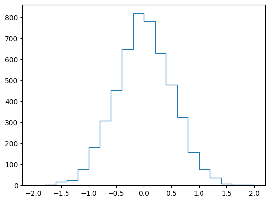

• Histograms can be cut down to size after filling
  • Shrink axis range with slices and using loc
  • Make binning coarser with rebin
  • See docs of boost-histogram or extended lecture
• Beyond 1D histograms
  • Supports advanced axis types (e.g. category axis)
  • Supports higher dimensional histograms
  • Supports generalized histograms with binned statistics (aka “profile” in ROOT)
  • See docs of boost-histogram or extended lecture

Fits

• Typical analysis work flow (often automated with Snakemake)

  1. Pre-select data
  2. Make histograms or profiles from pre-selected data
  3. Fit histograms or profiles to extract physical parameters

• Many specialized fitting tools for individual purposes, e.g.: scipy.optimize.curve_fit

• Generic libraries

  • RooFit
  • zfit
  • pyhf
  • iminuit
  • …

• Fitting (“estimation” in statistics)

  • Adjust parametric statistical model to dataset and find model parameters which match dataset best
  • AI community calls this “learning”
  • Estimate: result of fit

• Dataset: samples \(\{ \vec x_i \}\)

• Model: Probability density or probability mass function \(f(\vec x; \vec p)\) which depends on unknown parameters \(\vec p\)

• Conjecture: maximum-likelihood estimate (MLE) \(\hat{\vec p} = \text{argmax}_{\vec p} L(\vec p)\) is optimal, with \(L(\vec p) = \prod_i f(\vec x_i; \vec p)\)

  • Equivalent: minimize negative log-likelihood (NLL), \(\hat{\vec p} = \text{argmin}_{\vec p}(-\ln L(\vec p))\)

• Limiting case of maximum-likelihood fit: least-squares fit aka chi-square fit

• Python frontend to Minuit2 C++ library maintained by ROOT team at CERN
• Maximum-likelihood and least-squares fits with error estimation

import iminuit
from iminuit import Minuit
iminuit.__version__

'2.25.2'

• iminuit vs. other packages
  • pyhf
    • Better choice when you need to compute limits and preserve the likelihood
  • zfit and RooFit
    • Help you build statistical models: automatic normalization & convolutions
      • This has to be done “by hand” in iminuit
    • Good for standard tasks, but restrict your freedom
  • iminuit
    • Has good documentation
    • Well-designed API
    • Is very flexible and open
    • Is very fast with numba
• Typical fit in particle physics: mass distribution of decay candidates with signal peak over smooth background
• Task: fit signal fraction to calculate signal yield (fraction * number of candidates)

# fast implementations of statistical distributions, API similar to scipy.stats
import numba_stats
from numba_stats import norm, truncexpon
numba_stats.__version__

'1.7.0'

def make_data(size, seed=0):
    z=0.5
    mu=0.5
    sigma=0.1
    slope=0.5
    s = norm.rvs(mu, sigma, size=int(z * size), random_state=seed)
    b = truncexpon.rvs(0, 1, 0, slope, size=int((1-z) * size), random_state=seed)
    return np.append(s, b)

x1 = make_data(10_000)
plt.hist(x1, bins=100);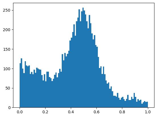

• Statistical model assumptions
  • Full sample is additive mixture of signal sample and background sample
  • Signal is normal-distributed; pdf is \(\mathcal{N}(\mu, \sigma)\) with parameters \(\mu\) and \(\sigma\)
  • Background is truncated exponential distribution

# model pdf
def model1(x, z, mu, sigma, slope):
    s = norm.pdf(x, mu, sigma)
    b = truncexpon.pdf(x, 0.0, 1.0, 0.0, slope)
    return (1 - z) * b + z * s

# we use NLL implementation provided by iminuit for convenience
from iminuit.cost import UnbinnedNLL

nll1 = UnbinnedNLL(x1, model1)
m = Minuit(nll1, z=0.5, mu=0.5, sigma=0.1, slope=1)

# need to set parameter limits or fit might fail
m.limits["z", "mu"] = (0, 1)
m.limits["sigma", "slope"] = (0, None)
m.migrad()

Migrad
FCN = -4741	Nfcn = 99
EDM = 2.03e-05 (Goal: 0.0002)
Valid Minimum	Below EDM threshold (goal x 10)
No parameters at limit	Below call limit
Hesse ok	Covariance accurate

	Name	Value	Hesse Error	Minos Error-	Minos Error+	Limit-	Limit+	Fixed
0	z	0.489	0.009			0	1
1	mu	0.4983	0.0020			0	1
2	sigma	0.0977	0.0019			0
3	slope	0.505	0.016			0

	z	mu	sigma	slope
z	8.48e-05	-2e-6 (-0.102)	9e-6 (0.535)	-0.06e-3 (-0.395)
mu	-2e-6 (-0.102)	3.94e-06	-0e-6 (-0.124)	-5e-6 (-0.153)
sigma	9e-6 (0.535)	-0e-6 (-0.124)	3.7e-06	-9e-6 (-0.280)
slope	-0.06e-3 (-0.395)	-5e-6 (-0.153)	-9e-6 (-0.280)	0.000268

Exercise

• Use interactive mode via m.interactive() to check how fit reacts to parameter changes
• Useful for debugging and to find starting values by hand

# do exercise here

• you can compute 2D confidence regions with Minuit.mncontour

Exercise * Draw the likelihood profile contour of parameters z and sigma with Minuit.draw_mncontour * Compute matrix of likelihood profile contours with Minuit.draw_mnmatrix

# do exercise here

Faster fits?

• Option 1: accelerate NLL computation with numba
• Option 2: use binned data

x2 = make_data(1_000_000)

• Option 1
  • NLL computation is trivially parallelizable: log(pdf) computed independently for each data point
  • Numba allows us to exploit auto-vectorization (SIMD instructions) and parallel computing on multiple cores
  • See full lecture for an example to numba-JIT compile the NLL function
  • See benchmark of iminuit + numba vs. RooFit
• Option 2
  • Often simpler: fit histograms
  • No bias from fitting histograms if done correctly, only loss in precision
  • Need model cdf instead of model pdf: \(F(x; \vec p) = \int_{-\infty}^x f(x'; \vec p) \text{d}x'\)

from iminuit.cost import BinnedNLL

# model is now a cdf!
def model3(x, z, mu, sigma, slope):
    s = norm.cdf(x, mu, sigma)
    b = truncexpon.cdf(x, 0.0, 1.0, 0.0, slope)
    return z * s + (1 - z) * b

w, xe = np.histogram(x2, bins=100, range=(0, 1))
nll3 = BinnedNLL(w, xe, model3)

m = Minuit(nll3, z=0.5, mu=0.5, sigma=1, slope=1)
m.migrad()

Migrad
FCN = 94.55 (χ²/ndof = 1.0)	Nfcn = 192
EDM = 1.76e-07 (Goal: 0.0002)
Valid Minimum	Below EDM threshold (goal x 10)
No parameters at limit	Below call limit
Hesse ok	Covariance accurate

	Name	Value	Hesse Error	Minos Error-	Minos Error+	Limit-	Limit+	Fixed
0	z	501.0e-3	0.9e-3
1	mu	500.3e-3	0.2e-3
2	sigma	100.06e-3	0.20e-3
3	slope	0.4982	0.0017

	z	mu	sigma	slope
z	8.91e-07	-0.02e-6 (-0.103)	0.10e-6 (0.557)	-0.7e-6 (-0.422)
mu	-0.02e-6 (-0.103)	4.03e-08	-0 (-0.125)	-0.05e-6 (-0.155)
sigma	0.10e-6 (0.557)	-0 (-0.125)	3.98e-08	-0.10e-6 (-0.307)
slope	-0.7e-6 (-0.422)	-0.05e-6 (-0.155)	-0.10e-6 (-0.307)	2.72e-06

• See study of binned fits vs. unbinned fit for detailed comparison
• With sufficient many bins (>= 20 in this case), increase in parameter uncertainties remains negligible
• Binned fits are (100-200)x faster than unbinned fits without using numba

Other fits

• To fit yields (counts) instead of fractions, use ExtendedUnbinnedNLL or ExtendedBinnedNLL
• To fit (x, y) pairs, use LeastSquares
• To fit simulated templates, use Template
• See documentation how models should be constructed then

Template fits

• Sometimes PDF/CDF not known in parametric form, but can be Monte-Carlo simulated
• Ansatz: Fit a histogram of simulation output (template) to data histogram
• Additional source of uncertainty from finite size of simulation
• Correct error propagation with Barlow-Beeston method, Barlow and Beeston, Comput.Phys.Commun. 77 (1993) 219-228
• iminuit.cost.Template
  • Extension to (s)weighted data and simuation, H. Dembinski, A. Abdelmotteleb, Eur.Phys.J.C 82 (2022) 11, 1043
  • Fast approximation to Barlow-Beeston method for unweighted data
  • Allows you to mix parametric models and templates

def make_data2(rng, nmc, truth, bins):
    xe = np.linspace(0, 1, bins + 1)
    b = np.diff(truncexpon.cdf(xe, 0, 1, 0, 1))
    s = np.diff(norm.cdf(xe, 0.5, 0.05))
    n = rng.poisson(b * truth[0]) + rng.poisson(s * truth[1])
    t = np.array([rng.poisson(b * nmc), rng.poisson(s * nmc)])
    return xe, n, t

rng = np.random.default_rng(1)
truth = 750, 250
xe, n, t = make_data2(rng, 200, truth, 15)

_, ax = plt.subplots(1, 2, figsize=(10, 4))
ax[0].stairs(n, xe, color="k", label="data")
ax[0].legend();
ax[1].stairs(t[0], xe, label="background")
ax[1].stairs(t[1], xe, label="signal")
ax[1].legend(title="templates");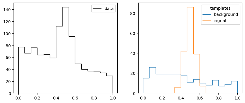

from iminuit.cost import Template

c = Template(n, xe, t)
m = Minuit(c, 1, 1)
m.migrad()

Migrad
FCN = 8.352 (χ²/ndof = 0.6)	Nfcn = 132
EDM = 2.75e-07 (Goal: 0.0002)
Valid Minimum	Below EDM threshold (goal x 10)
No parameters at limit	Below call limit
Hesse ok	Covariance accurate

	Name	Value	Hesse Error	Minos Error-	Minos Error+	Limit-	Limit+	Fixed
0	x0	770	70			0
1	x1	220	40			0

	x0	x1
x0	4.3e+03	-0.8e3 (-0.354)
x1	-0.8e3 (-0.354)	1.32e+03

• With Template you can also fit a mix of template and parametric model
• Often template only needed for background(s)

Exercise

• With make_data2 generate templates with 1 000 000 simulated points
• Fit this data with the Template cost function
• Compare parameter uncertainties

# do exercise here