LHCb Starter Kit 2023: Statistics I (extended version)

Hans Dembinski, TU Dortmund

• Scikit-HEP project
• Reading simple ROOT files
• Histograms
• Data visualization
• Fitting

About me

• Working with the LHCb experiment since 2016
• Before astroparticle physicist working with Pierre Auger Observatory and IceCube
• Statistics convener in LHCb (2019-2021, 2024-now)
• Interests
  • Statistics
  • High-performance computing
  • API design: “Make Interfaces Easy to Use Correctly and Hard to Use Incorrectly” Scott Meyers

Scikit-HEP project

• Provides high-performance data analysis tools in Python
• Partially funded by NSF grants
• Many LHCb developers: Eduardo Rodrigues, Chris Burr, myself, …
• Core values
  • Specialized tools that integrate well with existing Python ecosystem
  • Easy to use for beginners
  • Flexible for power users
  • Good documentation
  • Easy installation

The power of combinatorics

Build everything from basic components that fit together

Image credit: Toni Zaat on Unsplash

Important packages

• Python scientific stack

  • Numpy: fast computation with arrays
  • Scipy: integration, statistical distributions, special functions, …
  • Matplotlib: scientific plotting
  • Numba: JIT Compiler for Python (very fast)
  • Pandas: Convenient processing of tabular data

• Scikit-HEP Project

  • uproot: fast reading and writing of ROOT Trees
  • particle: get particle properties from PDG IDs
  • boost-histogram: multi-dimensional generalised histograms
  • iminuit: fitting and error computation package
  • resample: Easy bootstrapping to compute uncertainty and bias
  • pyhf: for histogram fitting/limit setting and preserving likelihoods

• Other packages

  • jacobi: Easy numerical error propagation
  • numba-stats: Fast statistical distributions for fitting
  • tabulate: Convert data tables to various formats (LaTeX, HTML, Markdown, …)
  • scikit-learn: Basic machine learning tools
  • xgboost: Gradient-boosting machine library that won many Kaggle competitions

Install everything with pip install LIBRARY

Working with Jupyter notebooks

• I recommend to use vscode
  • Very good Jupyter notebook support
  • Remote explorer: edit and run code on remote machines

Prepare computing environment

• In terminal, create and enter virtual environment (you need Python-3.8 or later)

  python3 -m venv .venv
  source .venv/bin/activate

• Install packages

  python -m pip install --upgrade numba matplotlib uproot boost-histogram iminuit scipy particle numba_stats ipywidgets

• uproot provides fast and convenient access to ROOT trees

import uproot

print(f"uproot {uproot.__version__}")

uproot 5.2.2

f = uproot.open("example.root")
event = f["event"]
 
event.show()

name                 | typename                 | interpretation                
---------------------+--------------------------+-------------------------------
trk_len              | int32_t                  | AsDtype('>i4')
mc_trk_len           | int32_t                  | AsDtype('>i4')
trk_imc              | int32_t[]                | AsJagged(AsDtype('>i4'))
trk_px               | float[]                  | AsJagged(AsDtype('>f4'))
trk_py               | float[]                  | AsJagged(AsDtype('>f4'))
trk_pz               | float[]                  | AsJagged(AsDtype('>f4'))
mc_trk_px            | float[]                  | AsJagged(AsDtype('>f4'))
mc_trk_py            | float[]                  | AsJagged(AsDtype('>f4'))
mc_trk_pz            | float[]                  | AsJagged(AsDtype('>f4'))
mc_trk_pid           | int32_t[]                | AsJagged(AsDtype('>i4'))

• Tree contains fake simulated LHCb events

• Truth in simulation

  • mc_trk_len: number of true particles in event
  • mc_trk_px: x-component of true momentum of particle
  • mc_trk_py: y-component of true momentum of particle
  • mc_trk_pz: z-component of true momentum of particle
  • mc_trk_pid: particle ID (PDG ID)

• Reconstructed simulation

  • trk_len: number reconstructed tracks in event
  • trk_px: x-component of momentum of reconstructed track
  • trk_py: y-component of momentum of reconstructed track
  • trk_pz: z-component of momentum of reconstructed track

• Special

  • trk_imc: index of matched true particle or -1

# get branches as arrays
arr = event.arrays(["trk_len", "trk_px", "mc_trk_len", "mc_trk_px"])

trk_len = arr["trk_len"]
trk_px = arr["trk_px"]
mc_trk_len = arr["mc_trk_len"]
mc_trk_px = arr["mc_trk_px"]

trk_len

[6,
 7,
 2,
 6,
 7,
 7,
 6,
 7,
 4,
 6,
 ...,
 2,
 4,
 13,
 3,
 6,
 3,
 4,
 6,
 3]
------------------
type: 1000 * int32

Exercise: Explore some other arrays from event

# do exercise here

• Some branches are 2D (e.g. trk_px)
• First index iterates over events
• Second index iterates over tracks per event

for ievent in range(5):
    print(ievent, trk_len[ievent], trk_px[ievent])

0 6 [-0.979, 0.232, -0.464, 0.629, 0.0287, 0.156]
1 7 [-0.59, 0.102, -0.282, -0.585, 0.0525, -0.249, -0.0836]
2 2 [0.124, 0.309]
3 6 [-0.287, 0.0082, -0.671, -0.933, -0.011, 0.0323]
4 7 [-0.086, -0.101, 0.0523, 0.204, -0.0287, 0.115, 0.0954]

• Mathematical operators and slicing works on these arrays similar to Numpy

trk_len[:10]

[6,
 7,
 2,
 6,
 7,
 7,
 6,
 7,
 4,
 6]
----------------
type: 10 * int32

trk_len > 10

[False,
 False,
 False,
 False,
 False,
 False,
 False,
 False,
 False,
 False,
 ...,
 False,
 False,
 True,
 False,
 False,
 False,
 False,
 False,
 False]
-----------------
type: 1000 * bool

• Many numpy functions work on awkward arrays

import numpy as np
print(np.__version__)

1.24.4

np.sum(trk_len)

5032

Exercise

• Use numpy functions to count how many events have zero tracks
• Hint: use np.sum and array mask

# do exercise here

# solution

f"{np.sum(trk_len == 0)} events with zero tracks"

'5 events with zero tracks'

# let's plot some things
import matplotlib.pyplot as plt

plt.hist(trk_len);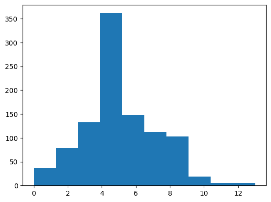

• For some operations and awkward arrays, we need the awkward library

import awkward as ak
print(ak.__version__)

2.6.1

Exercise * Try to plot trk_px * Can you figure out from the error message why it does not work? * Fix the issue with the function ak.flatten

# do exercise here

# solution

# plt.hist(trk_px) fails with helpful error message
plt.hist(ak.flatten(trk_px));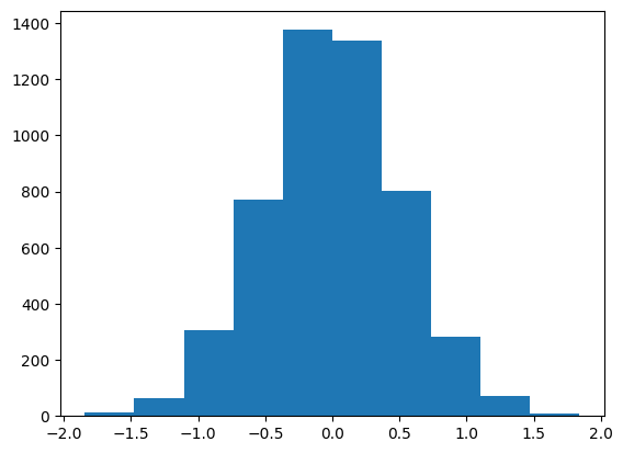

Reading data from a large tree

• Tree often do not fit into memory (tree size > 100 GB and more possible)
• Iterate over chunks

for chunk in event.iterate(["trk_px", "mc_trk_px"]):

    plt.hist(ak.flatten(chunk["trk_px"]), label="rec")
    plt.hist(ak.flatten(chunk["mc_trk_px"]), label="gen")
    plt.xlabel("px / MeVc-1")
    plt.legend()

    # stop after reading one chunk
    break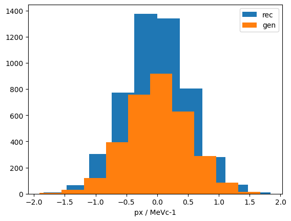

Accelerate Python code with Numba

• Just-In-Time compiler for scientific Python code
• Very powerful and very fast
• Fast for loops
• Not all Python code supported, works best with numerical code
• Only use when needed

import numba as nb
print(f"numba {nb.__version__}")

numba 0.57.1

• let’s subtract reconstructed from true momentum to check momentum resolution
• need to select tracks matched to MC particles
• this is relatively slow in Python, even if we use array computations

%%timeit -n 1 -r 3

delta_px = []
for chunk in event.iterate(["trk_px", "trk_imc", "mc_trk_px"]):
    for px, imc, mc_px in zip(chunk["trk_px"], chunk["trk_imc"], chunk["mc_trk_px"]):
        # select only tracks with associated true particle
        mask = imc >= 0
        subset_px = px[mask]
        subset_mc_px = mc_px[imc[mask]]
        # conversion to numpy needed
        delta_px = np.append(delta_px, subset_px - subset_mc_px) 

963 ms ± 35.4 ms per loop (mean ± std. dev. of 3 runs, 1 loop each)

# awkward arrays can be used in Numba

@nb.njit
def calc(chunk):
    r = []
    # loop over events
    for px, imc, mc_px in zip(chunk["trk_px"], chunk["trk_imc"], chunk["mc_trk_px"]):
        # loop over reconstructed tracks per event
        for px_i, imc_i in zip(px, imc):
            if imc_i < 0:
                continue
            mc_px_i = mc_px[imc_i]
            r.append(px_i - mc_px_i)
    return r

# function is JIT-compiled on first call with new data types
for chunk in event.iterate(["trk_px", "trk_imc", "mc_trk_px"]):
    calc(chunk)
    break

%%timeit -n 1 -r 3
delta_px = []
for data in event.iterate(["trk_px", "trk_imc", "mc_trk_px"]):
    d = calc(data)
    delta_px = np.append(delta_px, d)

4.17 ms ± 1.17 ms per loop (mean ± std. dev. of 3 runs, 1 loop each)

• Created array delta_px could still become very large in memory
• Better: Create histogram object first and then fill iteratively with chunks

• Python frontend to Boost.Histogram library in C++ from the Boost project
• Very fast and flexible
• Multi-dimensional histograms and other binned statistics (profiles!)
• Supports weighted data
• And much much more, see docs

import boost_histogram as bh
print(f"boost-histogram {bh.__version__}")

boost-histogram 1.4.0

# make an axis
xaxis = bh.axis.Regular(20, -2, 2)

# easy to make several histograms with same binning by reusing axis
h_px = bh.Histogram(xaxis)
h_mc_px = bh.Histogram(xaxis)

# let's use a finer binning for this one
h_delta_px = bh.Histogram(bh.axis.Regular(100, -2, 2))

# incremental filling
for data in event.iterate(["trk_px", "trk_imc", "mc_trk_px"]):
    h_px.fill(ak.flatten(trk_px))

h_px

Histogram(Regular(20, -2, 2), storage=Double()) # Sum: 5032.0

print(h_px)

                 ┌───────────────────────────────────────────────────────────┐
[-inf,   -2) 0   │                                                           │
[  -2, -1.8) 1   │▏                                                          │
[-1.8, -1.6) 3   │▎                                                          │
[-1.6, -1.4) 17  │█▎                                                         │
[-1.4, -1.2) 25  │█▊                                                         │
[-1.2,   -1) 78  │█████▌                                                     │
[  -1, -0.8) 181 │████████████▉                                              │
[-0.8, -0.6) 308 │█████████████████████▊                                     │
[-0.6, -0.4) 453 │████████████████████████████████▏                          │
[-0.4, -0.2) 647 │█████████████████████████████████████████████▉             │
[-0.2,    0) 819 │██████████████████████████████████████████████████████████ │
[   0,  0.2) 782 │███████████████████████████████████████████████████████▍   │
[ 0.2,  0.4) 629 │████████████████████████████████████████████▌              │
[ 0.4,  0.6) 480 │██████████████████████████████████                         │
[ 0.6,  0.8) 323 │██████████████████████▉                                    │
[ 0.8,    1) 159 │███████████▎                                               │
[   1,  1.2) 77  │█████▌                                                     │
[ 1.2,  1.4) 37  │██▋                                                        │
[ 1.4,  1.6) 7   │▌                                                          │
[ 1.6,  1.8) 3   │▎                                                          │
[ 1.8,    2) 3   │▎                                                          │
[   2,  inf) 0   │                                                           │
                 └───────────────────────────────────────────────────────────┘

# plot histogram with plt.stairs
plt.stairs(h_px.values(), h_px.axes[0].edges);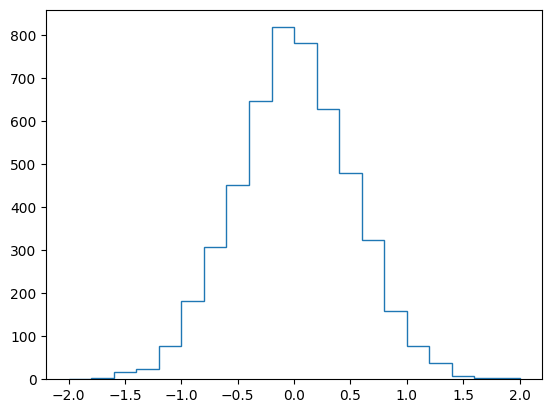

Exercise * Use iterative loop to fill h_mc_px and h_delta_px, use calc from before * Plot all three histograms overlaid into one figure with plt.stairs

# do exercise here

# solution

for chunk in event.iterate(["trk_px", "trk_imc", "mc_trk_px"]):
    h_px.fill(ak.flatten(chunk["trk_px"]))
    h_mc_px.fill(ak.flatten(chunk["trk_px"]))
    h_delta_px.fill(calc(chunk))
    
for h, label in ((h_px, "px"), (h_mc_px, "mc_px"), (h_delta_px, "delta_px")):
    plt.stairs(h.values(), h.axes[0].edges, label=label)
    
plt.legend();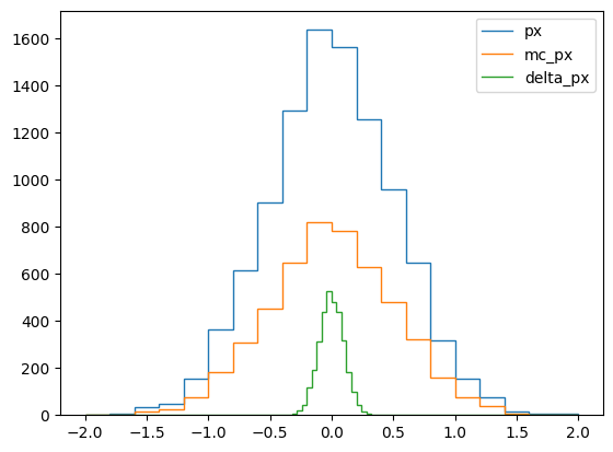

• Histograms can be reduced
• Shrink axis range with slices and using loc
• Make binning coarser with rebin

from boost_histogram.tag import loc, rebin

h_delta_px_2 = h_delta_px[loc(-0.5):loc(0.5):rebin(2)]

for h in (h_delta_px_2, h_delta_px):
    plt.stairs(h.values(), h.axes[0].edges,
               label=f"{len(h.values())} bins")
plt.legend();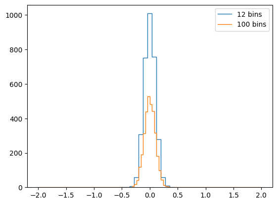

Beyond 1D histograms

• Supports advanced axis types (e.g. category axis)
• Supports higher dimensional histograms
• Supports generalized histograms with binned statistics (aka “profile” in ROOT)

# check detector momentum resolution in x for different particle species

p_axis = bh.axis.Regular(50, -2, 2)
pid_axis = bh.axis.IntCategory([], growth=True)

# profile: compute mean of reconstructed px in bins of mc_px for different particle species

p_2d = bh.Histogram(p_axis, pid_axis, storage=bh.storage.Mean())

branches = ["trk_px", "trk_imc", "mc_trk_px", "mc_trk_pid"]
for data in event.iterate(branches):
    for px, imc, mc_px, mc_pid in zip(*(data[b] for b in branches)):
        # select only tracks with associated true particle
        mask = imc >= 0
        px = px[mask]
        associated = imc[mask]
        mc_px = mc_px[associated]
        mc_pid = mc_pid[associated]

        p_2d.fill(mc_px, mc_pid, sample=px)

p_2d

Histogram(
  Regular(50, -2, 2),
  IntCategory([-321, 211, 2212, -2212, -211, 321], growth=True),
  storage=Mean()) # Sum: Mean(count=3240, value=0.000433322, variance=0.263444)

• We use particle library to look-up properties of particles based on their particle ID
• Get name, mass, life-time, quark content, …

import particle
print(f"particle {particle.__version__}")

particle 0.23.1

pids = p_2d.axes[1]
for i, pid in enumerate(pids):
    part = particle.Particle.from_pdgid(pid)

    x = p_2d.axes[0].centers
    y = p_2d.values()[:, i]
    ye = p_2d.variances()[:, i] ** 0.5
    plt.errorbar(x, y, ye, fmt="o", label=f"${part.latex_name}$ pid={int(part.pdgid)}")

plt.xlabel("mc_px")
plt.ylabel("px")
plt.legend();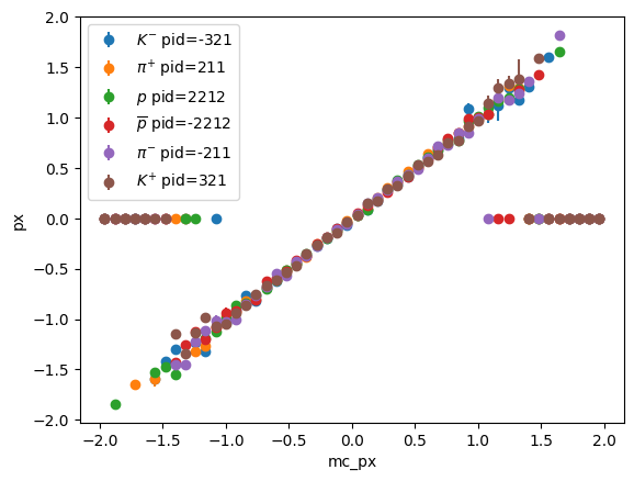

Exercise * Only show bins with sufficient entries, use p_2d.counts()

# do exercise here

# solution

pids = p_2d.axes[1]
for i, pid in enumerate(pids):
    part = particle.Particle.from_pdgid(pid)

    x = p_2d.axes[0].centers
    y = p_2d.values()[:, i]
    ye = p_2d.variances()[:, i] ** 0.5

    ma = (p_2d.counts() > 5)[:, i]
    
    plt.errorbar(x[ma], y[ma], ye[ma], fmt="o",
                 label=f"${part.latex_name}$ pid={int(part.pdgid)}")

plt.xlabel("mc_px")
plt.ylabel("px")
plt.legend();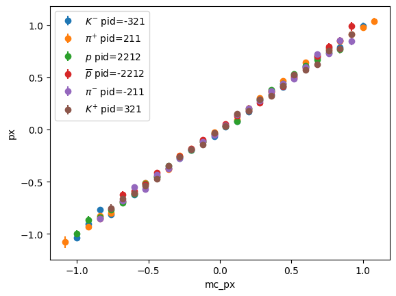

• We find that the reconstruction resolution is the same for all particle species
• Which means we can remove this axis by summing over its entries (called projection in ROOT)
• boost-histogram keeps track of events in overflow and underflow bins by default to make summing exact

p_1d = p_2d[:, sum] # remove PID axis by summing

x = p_1d.axes[0].centers
y = p_1d.values()
ye = p_1d.variances() ** 0.5
m = p_1d.counts() >= 5

plt.errorbar(x[m], y[m], ye[m], fmt="o")

plt.xlabel("mc_px")
plt.ylabel("px");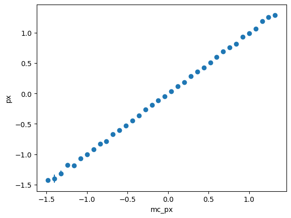

Fits

• Typical analysis work flow (often automated with Snakemake)

  1. Pre-select data
  2. Make histograms or profiles from pre-selected data
  3. Fit histograms or profiles to extract physical parameters

• Many specialized fitting tools for individual purposes, e.g.: scipy.optimize.curve_fit

• Generic libraries

  • RooFit
  • zfit
  • pyhf
  • iminuit
  • …

• Fitting (“estimation” in statistics)

  • Adjust parametric statistical model to dataset and find model parameters which match dataset best
  • AI community calls this “learning”
  • Estimate: result of fit

• Dataset: samples \(\{ \vec x_i \}\)

  • Sample can be one-dimensional or multidimensional
  • Values can be continuous (e.g. candidate mass) or discrete (e.g. bin counts)

• Model: Probability density or probability mass function \(f(\vec x; \vec p)\) which depends on unknown parameters \(\vec p\)

• Conjecture: maximum-likelihood estimate (MLE) \(\hat{\vec p} = \text{argmax}_{\vec p} L(\vec p)\) is optimal, with \(L(\vec p) = \prod_i f(\vec x_i; \vec p)\)

  • Proven: Asymptotically optimal, unbiased with minimum variance
    • No proof for finite data sets, but unchallenged
  • Universal: MLE can be computed for any problem
  • Equivalent: minimize negative log-likelihood (NLL), \(\hat{\vec p} = \text{argmin}_{\vec p}(-\ln L(\vec p))\)

• Limiting case of maximum-likelihood fit: least-squares fit aka chi-square fit

• Python frontend to Minuit2 C++ library maintained by ROOT team at CERN
• Maximum-likelihood and least-squares fits with error estimation
• Easy to use for beginners, flexible for power users
• Comes with builtin cost functions for common fits
• Large number of tutorials

import iminuit
from iminuit import Minuit

print(f"iminuit {iminuit.__version__}")

iminuit 2.25.2

iminuit vs. other packages

• pyhf
  • Better choice when you need to compute limits and preserve the likelihood
• zfit and RooFit
  • Help you build statistical models: automatic normalization & convolutions
    • This has to be done “by hand” in iminuit
  • Good for standard tasks, but restrict your freedom
• iminuit
  • Has good documentation
  • Well-designed API
  • Is very flexible and open
  • Is very fast with numba
• Typical fit in particle physics: mass distribution of decay candidates with signal peak over smooth background
• Task: get the number of signal candidates = signal yield
• Can be solved with a fit

def make_data(size, seed=1):
    rng = np.random.default_rng(seed)
    s = rng.normal(0.5, 0.1, size=size // 2)
    b = rng.exponential(1, size=2 * size)
    b = b[b < 1]
    b = b[: size // 2]
    x = np.append(s, b)
    return x

x1 = make_data(10_000)
plt.hist(x1, bins=100);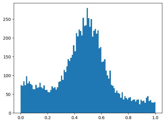

• To apply maximum-likelihood method, we need statistical model
• Full sample is additive mixture of signal sample and background sample
• Assumption 1: signal is normal-distributed; pdf is \(\mathcal{N}(\mu, \sigma)\) with parameters \(\mu\) and \(\sigma\)
• Assumption 2: background is truncated exponential distribution

# fast implementations of statistical distributions, API similar to scipy.stats
from numba_stats import norm, truncexpon

# model pdf
def model1(x, z, mu, sigma, slope):
    s = norm.pdf(x, mu, sigma)
    b = truncexpon.pdf(x, 0.0, 1.0, 0.0, slope)
    return (1 - z) * b + z * s

# negative log-likelihood
def nll1(z, mu, sigma, slope):
    logL = np.log(model1(x1, z, mu, sigma, slope))
    return -np.sum(logL)

m = Minuit(nll1, z=0.5, mu=0.5, sigma=1, slope=1)
m.errordef = Minuit.LIKELIHOOD
m.migrad()

Migrad
FCN = -1790	Nfcn = 209
EDM = 762 (Goal: 0.0001)
INVALID Minimum	ABOVE EDM threshold (goal x 10)
No parameters at limit	Below call limit
Hesse ok	Covariance accurate

	Name	Value	Hesse Error	Minos Error-	Minos Error+	Limit-	Limit+	Fixed
0	z	0.500	0.012
1	mu	0.500	0.003
2	sigma	0.155	0.005
3	slope	1.00	0.07

	z	mu	sigma	slope
z	0.000149	-1e-6 (-0.037)	0.033e-3 (0.508)	-0.25e-3 (-0.304)
mu	-1e-6 (-0.037)	9.19e-06	-0e-6 (-0.025)	-68e-6 (-0.335)
sigma	0.033e-3 (0.508)	-0e-6 (-0.025)	2.91e-05	-0.053e-3 (-0.147)
slope	-0.25e-3 (-0.304)	-68e-6 (-0.335)	-0.053e-3 (-0.147)	0.00442

• Fit did not work
• Plotting 1D or 2D slices of likelihood may help

m.draw_profile("z");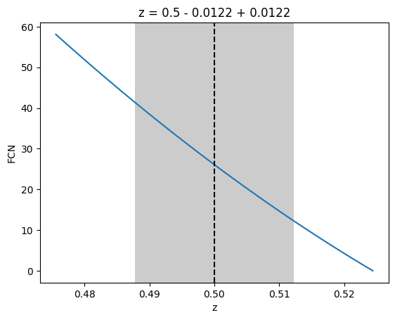

• Increase print level

m.print_level = 1
m.migrad()
m.print_level = 0

W FCN result is NaN for [ 0.406325 0.495731 -0.0437361 1.13819 ]
W FCN result is NaN for [ nan nan nan nan ]
W FCN result is NaN for [ nan nan nan nan ]
W FCN result is NaN for [ nan nan nan nan ]
W FCN result is NaN for [ nan nan nan nan ]
W FCN result is NaN for [ nan nan nan nan ]
W FCN result is NaN for [ nan nan nan nan ]
W FCN result is NaN for [ nan nan nan nan ]
W FCN result is NaN for [ nan nan nan nan ]
W FCN result is NaN for [ nan nan nan nan ]
W FCN result is NaN for [ nan nan nan nan ]
W VariableMetricBuilder No improvement in line search
W VariableMetricBuilder Iterations finish without convergence; Edm 761.614 Requested 0.0001
W VariableMetricBuilder No convergence; Edm 761.614 is above tolerance 0.001
W FCN result is NaN for [ 0.406325 0.495731 -0.0437361 1.13819 ]
W FCN result is NaN for [ nan nan nan nan ]
W FCN result is NaN for [ nan nan nan nan ]
W FCN result is NaN for [ nan nan nan nan ]
W FCN result is NaN for [ nan nan nan nan ]
W FCN result is NaN for [ nan nan nan nan ]
W FCN result is NaN for [ nan nan nan nan ]
W FCN result is NaN for [ nan nan nan nan ]
W FCN result is NaN for [ nan nan nan nan ]
W FCN result is NaN for [ nan nan nan nan ]
W FCN result is NaN for [ nan nan nan nan ]
W VariableMetricBuilder No improvement in line search
W VariableMetricBuilder Iterations finish without convergence; Edm 761.614 Requested 0.0001
W VariableMetricBuilder No convergence; Edm 761.614 is above tolerance 0.001
W FCN result is NaN for [ 0.406325 0.495731 -0.0437361 1.13819 ]
W FCN result is NaN for [ nan nan nan nan ]
W FCN result is NaN for [ nan nan nan nan ]
W FCN result is NaN for [ nan nan nan nan ]
W FCN result is NaN for [ nan nan nan nan ]
W FCN result is NaN for [ nan nan nan nan ]
W FCN result is NaN for [ nan nan nan nan ]
W FCN result is NaN for [ nan nan nan nan ]
W FCN result is NaN for [ nan nan nan nan ]
W FCN result is NaN for [ nan nan nan nan ]
W FCN result is NaN for [ nan nan nan nan ]
W VariableMetricBuilder No improvement in line search
W VariableMetricBuilder Iterations finish without convergence; Edm 761.614 Requested 0.0001
W VariableMetricBuilder No convergence; Edm 761.614 is above tolerance 0.001
W FCN result is NaN for [ 0.406325 0.495731 -0.0437361 1.13819 ]
W FCN result is NaN for [ nan nan nan nan ]
W FCN result is NaN for [ nan nan nan nan ]
W FCN result is NaN for [ nan nan nan nan ]
W FCN result is NaN for [ nan nan nan nan ]
W FCN result is NaN for [ nan nan nan nan ]
W FCN result is NaN for [ nan nan nan nan ]
W FCN result is NaN for [ nan nan nan nan ]
W FCN result is NaN for [ nan nan nan nan ]
W FCN result is NaN for [ nan nan nan nan ]
W FCN result is NaN for [ nan nan nan nan ]
W VariableMetricBuilder No improvement in line search
W VariableMetricBuilder Iterations finish without convergence; Edm 761.614 Requested 0.0001
W VariableMetricBuilder No convergence; Edm 761.614 is above tolerance 0.001
W FCN result is NaN for [ 0.406325 0.495731 -0.0437361 1.13819 ]
W FCN result is NaN for [ nan nan nan nan ]
W FCN result is NaN for [ nan nan nan nan ]
W FCN result is NaN for [ nan nan nan nan ]
W FCN result is NaN for [ nan nan nan nan ]
W FCN result is NaN for [ nan nan nan nan ]
W FCN result is NaN for [ nan nan nan nan ]
W FCN result is NaN for [ nan nan nan nan ]
W FCN result is NaN for [ nan nan nan nan ]
W FCN result is NaN for [ nan nan nan nan ]
W FCN result is NaN for [ nan nan nan nan ]
W VariableMetricBuilder No improvement in line search
W VariableMetricBuilder Iterations finish without convergence; Edm 761.614 Requested 0.0001
W VariableMetricBuilder No convergence; Edm 761.614 is above tolerance 0.001

• fit failed because parameters need limits

Exercise

• Repeat fit, but with parameter limits.
• Set parameter limits by calling m.limits["parameter"] = (lower, upper) before m.migrad()
• You can set identical limits for multiple parameters, for example, m.limits["a", "b"] = (0, 1)

# do exercise here

# solution

m.limits["z", "mu"] = (0, 1)
m.limits["sigma", "slope"] = (0, None)
m.migrad()

Migrad
FCN = -2095	Nfcn = 481
EDM = 1.78e-06 (Goal: 0.0001)
Valid Minimum	Below EDM threshold (goal x 10)
No parameters at limit	Below call limit
Hesse ok	Covariance accurate

	Name	Value	Hesse Error	Minos Error-	Minos Error+	Limit-	Limit+	Fixed
0	z	0.498	0.009			0	1
1	mu	0.4968	0.0020			0	1
2	sigma	0.0994	0.0020			0
3	slope	1.03	0.06			0

	z	mu	sigma	slope
z	8.94e-05	-1e-6 (-0.063)	10e-6 (0.547)	-0.12e-3 (-0.213)
mu	-1e-6 (-0.063)	4.21e-06	-0e-6 (-0.061)	-27e-6 (-0.225)
sigma	10e-6 (0.547)	-0e-6 (-0.061)	3.94e-06	-18e-6 (-0.156)
slope	-0.12e-3 (-0.213)	-27e-6 (-0.225)	-18e-6 (-0.156)	0.00345

• compute asymmetric errors with Minos algorithm (profile likelihood method)

m.minos()

Migrad
FCN = -2095	Nfcn = 692
EDM = 1.78e-06 (Goal: 0.0001)
Valid Minimum	Below EDM threshold (goal x 10)
No parameters at limit	Below call limit
Hesse ok	Covariance accurate

	Name	Value	Hesse Error	Minos Error-	Minos Error+	Limit-	Limit+	Fixed
0	z	0.498	0.009	-0.009	0.009	0	1
1	mu	0.4968	0.0021	-0.0020	0.0020	0	1
2	sigma	0.0994	0.0020	-0.0019	0.0020	0
3	slope	1.03	0.06	-0.06	0.06	0

	z		mu		sigma		slope
Error	-0.009	0.009	-0.002	0.002	-0.0019	0.0020	-0.06	0.06
Valid	True	True	True	True	True	True	True	True
At Limit	False	False	False	False	False	False	False	False
Max FCN	False	False	False	False	False	False	False	False
New Min	False	False	False	False	False	False	False	False

	z	mu	sigma	slope
z	8.94e-05	-1e-6 (-0.063)	10e-6 (0.547)	-0.12e-3 (-0.213)
mu	-1e-6 (-0.063)	4.21e-06	-0e-6 (-0.061)	-27e-6 (-0.225)
sigma	10e-6 (0.547)	-0e-6 (-0.061)	3.94e-06	-18e-6 (-0.156)
slope	-0.12e-3 (-0.213)	-27e-6 (-0.225)	-18e-6 (-0.156)	0.00345

• you can compute 2D confidence regions with mncontour and draw them with draw_mncontour

m.draw_mncontour("z", "sigma");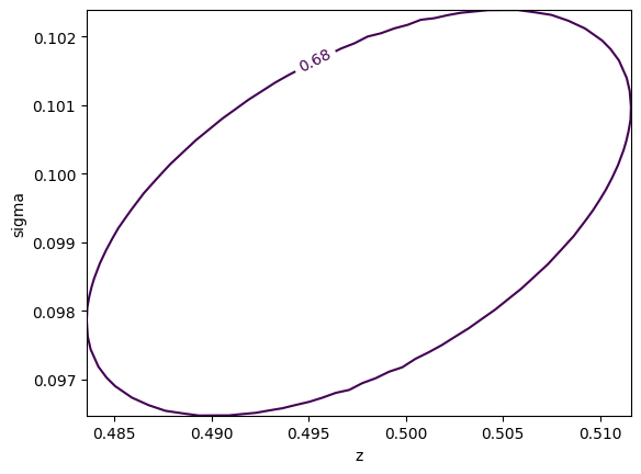

Exercise

• Draw 1,2,3 sigma contours, use keyword cl

# do exercise here

# solution

m.draw_mncontour("z", "sigma", cl=(1, 2, 3));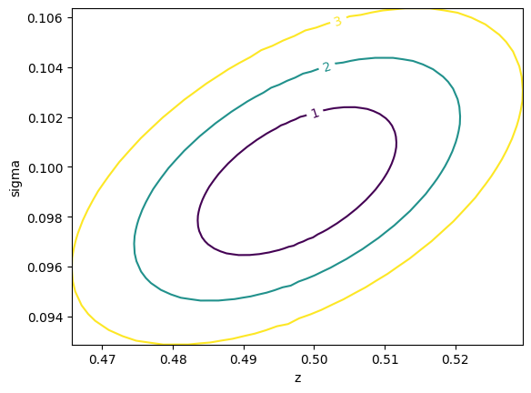

• for nice overview: compute matrix of likelihood profiles with draw_mnmatrix

m.draw_mnmatrix(figsize=(9,7));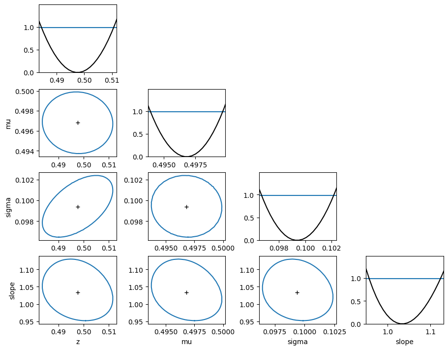

• Writing unbinned negative-log-likelihood is repetitive, only model ever changes
• Use built-in cost function from iminuit to get nice extras

from iminuit.cost import UnbinnedNLL

nll1 = UnbinnedNLL(x1, model1)
m = Minuit(nll1, z=0.5, mu=0.5, sigma=1, slope=1)
m.limits["z", "mu"] = (0, 1)
m.limits["sigma", "slope"] = (0, None)

m.migrad()

Migrad
FCN = -4189	Nfcn = 169
EDM = 8.37e-05 (Goal: 0.0002)	time = 0.4 sec
Valid Minimum	Below EDM threshold (goal x 10)
No parameters at limit	Below call limit
Hesse ok	Covariance accurate

	Name	Value	Hesse Error	Minos Error-	Minos Error+	Limit-	Limit+	Fixed
0	z	0.498	0.009			0	1
1	mu	0.4968	0.0020			0	1
2	sigma	0.0994	0.0020			0
3	slope	1.03	0.06			0

	z	mu	sigma	slope
z	8.62e-05	-1e-6 (-0.037)	10e-6 (0.529)	-0.11e-3 (-0.211)
mu	-1e-6 (-0.037)	4.17e-06	-0e-6 (-0.039)	-28e-6 (-0.230)
sigma	10e-6 (0.529)	-0e-6 (-0.039)	3.83e-06	-17e-6 (-0.152)
slope	-0.11e-3 (-0.211)	-28e-6 (-0.230)	-17e-6 (-0.152)	0.00345

Exercise

• Use interactive mode via m.interactive() to check how fit reacts to parameter changes
• Useful for debugging and to find starting values by hand

# do exercise here

Faster fits?

• Option 1: accelerate NLL computation with Numba
• Option 2: use binned data

x2 = make_data(1_000_000)

m = Minuit(UnbinnedNLL(x2, model1), z=0.5, mu=0.5, sigma=1, slope=1)
m.limits["z", "mu"] = (0, 1)
m.limits["sigma", "slope"] = (0, None)
m.migrad()

Migrad
FCN = -4.216e+05	Nfcn = 169
EDM = 0.000135 (Goal: 0.0002)	time = 5.9 sec
Valid Minimum	Below EDM threshold (goal x 10)
No parameters at limit	Below call limit
Hesse ok	Covariance accurate

	Name	Value	Hesse Error	Minos Error-	Minos Error+	Limit-	Limit+	Fixed
0	z	499.7e-3	0.9e-3			0	1
1	mu	499.98e-3	0.20e-3			0	1
2	sigma	99.59e-3	0.20e-3			0
3	slope	0.997	0.006			0

	z	mu	sigma	slope
z	8.87e-07	-0.01e-6 (-0.049)	0.10e-6 (0.548)	-1.2e-6 (-0.229)
mu	-0.01e-6 (-0.049)	4.18e-08	-0 (-0.060)	-0.26e-6 (-0.226)
sigma	0.10e-6 (0.548)	-0 (-0.060)	4.09e-08	-0.18e-6 (-0.164)
slope	-1.2e-6 (-0.229)	-0.26e-6 (-0.226)	-0.18e-6 (-0.164)	3.06e-05

General insights * Time spend in minimizer is negligible * Bottleneck is evaluating NLL function * Bottleneck inside NLL function is usually evaluation of model * NLL computation is trivially parallelizable: log(pdf) computed independently for each data point * Numba allows us to exploit auto-vectorization (SIMD instructions) and parallel computing on multiple cors

@nb.njit(parallel=True, fastmath=True, error_model="numpy")
def nll2(z, mu, sigma, slope):
    def model(x, z, mu, sigma, slope):
        s = norm.pdf(x, mu, sigma)
        b = truncexpon.pdf(x, 0.0, 1.0, 0.0, slope)
        return (1 - z) * b + z * s

    logL = np.log(model(x2, z, mu, sigma, slope))
    return -np.sum(logL)

# compile function
nll2(0.5, 0.5, 0.1, 0.1);

OMP: Info #276: omp_set_nested routine deprecated, please use omp_set_max_active_levels instead.

m = Minuit(nll2, z=0.5, mu=0.5, sigma=1, slope=1)
m.errordef = Minuit.LIKELIHOOD
m.limits["z", "mu"] = (0, 1)
m.limits["sigma", "slope"] = (0, None)
m.migrad()

Migrad
FCN = -2.108e+05	Nfcn = 242
EDM = 2.48e-06 (Goal: 0.0001)	time = 1.4 sec
Valid Minimum	Below EDM threshold (goal x 10)
No parameters at limit	Below call limit
Hesse ok	Covariance accurate

	Name	Value	Hesse Error	Minos Error-	Minos Error+	Limit-	Limit+	Fixed
0	z	499.7e-3	0.9e-3			0	1
1	mu	499.98e-3	0.20e-3			0	1
2	sigma	99.59e-3	0.20e-3			0
3	slope	0.997	0.006			0

	z	mu	sigma	slope
z	8.87e-07	-0.01e-6 (-0.049)	0.10e-6 (0.548)	-1.2e-6 (-0.229)
mu	-0.01e-6 (-0.049)	4.18e-08	-0 (-0.060)	-0.26e-6 (-0.226)
sigma	0.10e-6 (0.548)	-0 (-0.060)	4.09e-08	-0.18e-6 (-0.164)
slope	-1.2e-6 (-0.229)	-0.26e-6 (-0.226)	-0.18e-6 (-0.164)	3.06e-05

• Often simpler: fit histograms

• No bias from fitting histograms if done correctly, only loss in precision

• Need model cdf instead of model pdf: \(F(x; \vec p) = \int_{-\infty}^x f(x'; \vec p) \text{d}x'\)

• Recommended to use iminuit.cost.BinnedNLL, comes with many useful features

from iminuit.cost import BinnedNLL

# model is now a cdf!
def model3(x, z, mu, sigma, slope):
    s = norm.cdf(x, mu, sigma)
    b = truncexpon.cdf(x, 0.0, 1.0, 0.0, slope)
    return (1 - z) * b + z * s

w, xe = np.histogram(x2, bins=100, range=(0, 1))
nll3 = BinnedNLL(w, xe, model3)

m = Minuit(nll3, z=0.5, mu=0.5, sigma=1, slope=1)
m.migrad()

Migrad
FCN = 84.34 (χ²/ndof = 0.9)	Nfcn = 162
EDM = 1.36e-07 (Goal: 0.0002)	time = 0.4 sec
Valid Minimum	Below EDM threshold (goal x 10)
No parameters at limit	Below call limit
Hesse ok	Covariance accurate

	Name	Value	Hesse Error	Minos Error-	Minos Error+	Limit-	Limit+	Fixed
0	z	499.7e-3	0.9e-3
1	mu	499.99e-3	0.20e-3
2	sigma	99.58e-3	0.20e-3
3	slope	0.997	0.006

	z	mu	sigma	slope
z	8.98e-07	-0.01e-6 (-0.049)	0.10e-6 (0.535)	-1.2e-6 (-0.236)
mu	-0.01e-6 (-0.049)	4.22e-08	-0 (-0.052)	-0.26e-6 (-0.228)
sigma	0.10e-6 (0.535)	-0 (-0.052)	4.15e-08	-0.18e-6 (-0.161)
slope	-1.2e-6 (-0.236)	-0.26e-6 (-0.228)	-0.18e-6 (-0.161)	3.09e-05

• See study of binned fits vs. unbinned fit for detailed comparison
• With sufficient many bins (>= 20 in this case), increase in parameter uncertainties remains negligible
• Binned fits are (100-200)x faster than unbinned fits without using numba

How well is model matching data?

• Judgement requires binning of data
• Look at pull distribution
  • Compute (data - model) / error for each bin
• Compare \(\chi^2\) value (goodness-of-fit test statistic) against the degrees of freedom
  • Simple check: reduced chi-square \(\chi^2/n_\text{dof}\) should be about 1
  • Better check: p-value \(= \int_{\chi^2_\text{observed}}^{\infty} f(\chi^2; n_\text{dof}) \, \text{d}\chi^2\) (survival function)
  • If p-value very small (< 1%), wrong model or underestimated errors

from scipy.stats import chi2

pulls = nll3.pulls(m.values)
cx = xe[:-1] + np.diff(xe)
plt.errorbar(cx, pulls, np.ones_like(pulls), fmt="o");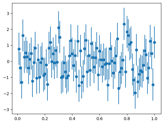

# m.fval is chi-square distributed for all built-in cost functions
# except UnbinnedNLL and ExtendedUnbinnedNLL
pvalue = chi2(m.ndof).sf(m.fval)
f"chi2/ndof = {m.fmin.reduced_chi2:.2f} p-value = {pvalue:.2f}"

'chi2/ndof = 0.88 p-value = 0.80'

Exercise

• Plot histogram of pulls, should look like standard normal distribution
• Compute mean and standard deviation (use np.mean and np.std)

# do exercise here

# solution

xe = plt.hist(pulls, bins=20)[1]
plt.title(f"mean = {np.mean(pulls):.2f} std = {np.std(pulls):.2f}");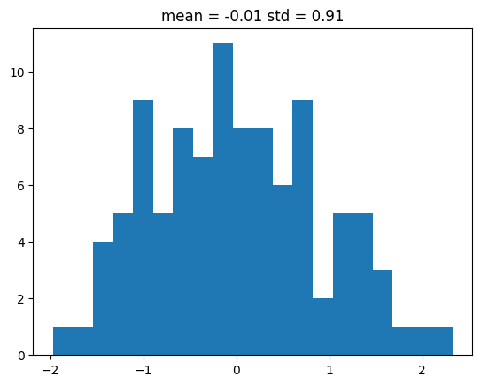

Other fits

• To fit yields (counts) instead of fractions, use ExtendedUnbinnedNLL or ExtendedBinnedNLL
• To fit (x, y) pairs, use LeastSquares
• To fit simulated templates, use Template
• See documentation how models should be constructed then

Template fits

• Sometimes PDF/CDF not known in parametric form, but can be Monte-Carlo simulated
• Idea: fit a histogram of simulation output (template) to data histogram
• Additional source of uncertainty from finite size of simulation
• Correct error propagation with Barlow-Beeston method, Barlow and Beeston, Comput.Phys.Commun. 77 (1993) 219-228
• iminuit.cost.Template
  • Extension to weighted data and simuation, H. Dembinski, A. Abdelmotteleb, Eur.Phys.J.C 82 (2022) 11, 1043
  • Approximation to Barlow-Beeston method for unweighted data
  • Faster computation
  • Allows you to mix parametric models and templates

def make_data2(rng, nmc, truth, bins):
    xe = np.linspace(0, 1, bins + 1)
    b = np.diff(truncexpon.cdf(xe, 0, 1, 0, 1))
    s = np.diff(norm.cdf(xe, 0.5, 0.05))
    n = rng.poisson(b * truth[0]) + rng.poisson(s * truth[1])
    t = np.array([rng.poisson(b * nmc), rng.poisson(s * nmc)])
    return xe, n, t

rng = np.random.default_rng(1)
truth = 750, 250
xe, n, t = make_data2(rng, 200, truth, 15)

_, ax = plt.subplots(1, 2, figsize=(10, 4))
ax[0].stairs(n, xe, color="k", label="data")
ax[0].legend();
ax[1].stairs(t[0], xe, label="background")
ax[1].stairs(t[1], xe, label="signal")
ax[1].legend(title="templates");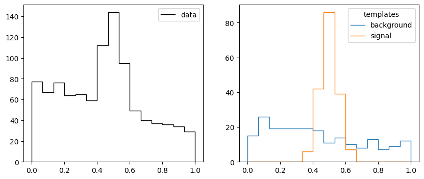

from iminuit.cost import Template

c = Template(n, xe, t)
m = Minuit(c, 1, 1)
m.migrad()

Migrad
FCN = 8.352 (χ²/ndof = 0.6)	Nfcn = 132
EDM = 2.75e-07 (Goal: 0.0002)	time = 0.5 sec
Valid Minimum	Below EDM threshold (goal x 10)
No parameters at limit	Below call limit
Hesse ok	Covariance accurate

	Name	Value	Hesse Error	Minos Error-	Minos Error+	Limit-	Limit+	Fixed
0	x0	770	70			0
1	x1	220	40			0

	x0	x1
x0	4.3e+03	-0.8e3 (-0.354)
x1	-0.8e3 (-0.354)	1.32e+03

Exercise

• With make_data2 generate templates with 1 000 000 simulated points
• Fit this data with the Template cost function
• Compare parameter uncertainties

# do exercise here

# solution

xe, n, t = make_data2(rng, 1_000_000, truth, 15)
c = Template(n, xe, t)
m = Minuit(c, 1, 1)
m.migrad()

Migrad
FCN = 4.329 (χ²/ndof = 0.3)	Nfcn = 110
EDM = 2.66e-06 (Goal: 0.0002)
Valid Minimum	Below EDM threshold (goal x 10)
No parameters at limit	Below call limit
Hesse ok	Covariance accurate

	Name	Value	Hesse Error	Minos Error-	Minos Error+	Limit-	Limit+	Fixed
0	x0	820	32			0
1	x1	201	20			0

	x0	x1
x0	1.03e+03	-0.2e3 (-0.326)
x1	-0.2e3 (-0.326)	415

• With Template you can also fit a mix of template and parametric model
• Often template only needed for background(s)

# density model for signal component, as for ExtendedBinnedNLL
def model5(x, s, mu, sigma):
    return s * norm.cdf(x, mu, sigma)

c = Template(n, xe, (t[0], model5))
m = Minuit(c, x0=700, x1_s=300, x1_mu=0.5, x1_sigma=0.1)
m.limits["x1_mu"] = (0, 1)
m.limits["x1_sigma"] = (0, None)

m.migrad()

Migrad
FCN = 2.526 (χ²/ndof = 0.2)	Nfcn = 106
EDM = 1.52e-06 (Goal: 0.0002)
Valid Minimum	Below EDM threshold (goal x 10)
No parameters at limit	Below call limit
Hesse ok	Covariance accurate

	Name	Value	Hesse Error	Minos Error-	Minos Error+	Limit-	Limit+	Fixed
0	x0	819	34			0
1	x1_s	202	23
2	x1_mu	0.492	0.006			0	1
3	x1_sigma	0.049	0.007			0

	x0	x1_s	x1_mu	x1_sigma
x0	1.16e+03	-0.3e3 (-0.428)	8.13e-3 (0.038)	-79.31e-3 (-0.330)
x1_s	-0.3e3 (-0.428)	541	-8.17e-3 (-0.056)	79.27e-3 (0.483)
x1_mu	8.13e-3 (0.038)	-8.17e-3 (-0.056)	3.99e-05	-0 (-0.069)
x1_sigma	-79.31e-3 (-0.330)	79.27e-3 (0.483)	-0 (-0.069)	4.98e-05

Overfitting

• Do not use models with degenerate parameters
• Avoid overfitting

from iminuit.cost import LeastSquares
from numba_stats import bernstein  # Bernstein polynomials > Chebychev polynomials

x = [-0.37, -0.25, -0.15, -0.05, 0.047, 0.147, 0.243, 0.374]
y = [0.96, 0.90, 0.85, 0.81, 0.75, 0.66, 0.42, 0.14]
ey = [0.01, 0.01, 0.01, 0.02, 0.02, 0.03, 0.04, 0.05]

def model(x, p):
    return bernstein.density(x, p, -0.4, 0.4)

start = np.ones(3)
m = Minuit(LeastSquares(x, y, ey, model), start)
m.migrad()

Migrad
FCN = 23.81 (χ²/ndof = 4.8)	Nfcn = 51
EDM = 4.25e-21 (Goal: 0.0002)
Valid Minimum	Below EDM threshold (goal x 10)
No parameters at limit	Below call limit
Hesse ok	Covariance accurate

	Name	Value	Hesse Error	Minos Error-	Minos Error+	Limit-	Limit+	Fixed
0	x0	0.950	0.011
1	x1	0.920	0.027
2	x2	0.21	0.04

	x0	x1	x2
x0	0.000127	-0.21e-3 (-0.680)	0.14e-3 (0.321)
x1	-0.21e-3 (-0.680)	0.000737	-0.7e-3 (-0.666)
x2	0.14e-3 (0.321)	-0.7e-3 (-0.666)	0.00147

Exercise

• Fit with increasing number of parameters (increase the length of the starting parameters)

  • What do you observe? Look out for changes in chi2/ndof and the parameter correlations

• Try fitting this model

  def model(x, p):
      return p[0] + bernstein.density(x, p[1:], -0.4, 0.4)

  • What do you observe?

# do exercise here

# solution

# def model(x, p):
#       return p[0] + bernstein.density(x, p[1:], -0.4, 0.4)

start = np.ones(6)
m = Minuit(LeastSquares(x, y, ey, model), start)
m.migrad()

Migrad
FCN = 1.069 (χ²/ndof = 0.5)	Nfcn = 152
EDM = 2.41e-15 (Goal: 0.0002)
Valid Minimum	Below EDM threshold (goal x 10)
No parameters at limit	Below call limit
Hesse ok	Covariance accurate

	Name	Value	Hesse Error	Minos Error-	Minos Error+	Limit-	Limit+	Fixed
0	x0	0.956	0.026
1	x1	1.02	0.13
2	x2	0.47	0.27
3	x3	1.30	0.34
4	x4	0.29	0.25
5	x5	0.10	0.08

	x0	x1	x2	x3	x4	x5
x0	0.000693	-3.0e-3 (-0.885)	5.7e-3 (0.800)	-6.2e-3 (-0.687)	3.6e-3 (0.551)	-0.7e-3 (-0.307)
x1	-3.0e-3 (-0.885)	0.0161	-0.033 (-0.961)	0.037 (0.852)	-0.022 (-0.698)	0.004 (0.394)
x2	5.7e-3 (0.800)	-0.033 (-0.961)	0.0721	-0.09 (-0.953)	0.05 (0.822)	-0.010 (-0.480)
x3	-6.2e-3 (-0.687)	0.037 (0.852)	-0.09 (-0.953)	0.116	-0.08 (-0.938)	0.016 (0.583)
x4	3.6e-3 (0.551)	-0.022 (-0.698)	0.05 (0.822)	-0.08 (-0.938)	0.062	-0.014 (-0.721)
x5	-0.7e-3 (-0.307)	0.004 (0.394)	-0.010 (-0.480)	0.016 (0.583)	-0.014 (-0.721)	0.00649