LHCb Starter Kit 2023: Statistics II (extended version)

Hans Dembinski, TU Dortmund

Uncertainties of estimators
Bootstrapping of uncertainties
Error propagation
Estimation of systematic uncertainties
Resources for further learning

What is an uncertainty, really?

Example: \(a = 3 \pm 0.5\), where 0.5 is the standard error (jargon: “error” = uncertainty).
What we would like it to mean: “The true value is between 2.5 and 3.5 with a probability of 68 %”.
What it technically means (in most cases): “The interval 2.5 to 3.5, if always constructed with the same procedure, contains the true value in 68 % of identically repeated random experiments.”
Both statements coincide only in the asymptotic limit of infinitely large samples.

Statistical and systematic uncertainties

Statistical uncertainty

Origin: We use finite sample instead of infinite distribution
Goes down as simple size increases
Example
- Arithmetic mean: \(\bar x = \frac 1N\sum_i x_i\)
- Variance of \(\bar x\): \(\hat V_{\bar x} = \frac{1}{N - 1} \frac 1 N\sum_i (x_i - \bar x)^2\)
We have reliable standard recipes to calculate these

Variance or standard deviation?

Standard deviation \(\sigma = \sqrt{V}\)
Variance is more fundamental
- Second central moment of distribution
- \(V = V_1 + V_2\), but \(\sigma = \sqrt{\sigma_1^2 + \sigma_2^2}\)
Communicate standard deviations, compute with variances

Systematic uncertainty

Origin: Imperfect appartus or technique, deviations of reality from simplified models
Quantifies potential mistakes in analysis
Does not go down as sample size increases
Often correlated
- Real-life: Measured the length of ten shoes with ruler than has factory tolerance of 0.1 mm
- LHCb: Measured cross-sections with value of luminosity that has uncertainty of 1-2%
Not well covered in statistics books, but some theoretical results available

Estimators

Estimator maps dataset to value \(\{x_i \} \to \hat p\)
- Notation: \(\hat p\) is estimate of true value \(p\)
- Estimator can have functional form or be an algorithm
- Arithmetic mean \(\hat \mu = \frac 1N \sum_i x_i\)
- Sample median: Sort \(x_i\), pick value in the middle
Many kinds of estimators, some better than others
Optimal estimators
- As close to true value as possible
- Easy to compute and/or easy to apply to any problem
- Robustness against outliers
In HEP, we mainly use
- Plug-in estimator
- Maximum-likelihood estimator (MLE)

Bias and variance

In one experiment, we obtain sample \(\{ x_i \}\) with size \(N\) and compute estimate \(\hat a\)
Sample \(\{ x_i \}\) is random, estimate \(\hat a\) also random
If experiment is identically repeated \(K\) times, we get sample \(\{ x_i \}_k\) and estimate \(\hat a_k\) each time
Derive accuracy of estimator from estimates \(\{ \hat a_1, \hat a_2, \dots, \hat a_K \}\)
- Bias of \(\hat a\) = \(\frac1K \sum_i (\hat a_i - a)\)
- Variance of \(\hat a\) = \(\frac1{K-1}\sum_i (\hat a_i - \frac 1 K \sum_k \hat a_k)^2\)
Example for a biased estimator: \(\hat V = \frac1N\sum_i (x_i - \hat\mu)^2\) is biased, if \(\hat \mu\) is estimated from same sample

from matplotlib import pyplot as plt
import numpy as np

mu = 1
sigma = 1

N = 10
K = 10000
var_1, var_2 = [], []
for k in range(K):
    rng = np.random.default_rng(seed=k)
    x_k = rng.normal(mu, sigma, size=N)
    v1 = np.var(x_k)
    v2 = np.mean((x_k - mu) ** 2)
    var_1.append(v1)
    var_2.append(v2)

fig, ax = plt.subplots(1, 2, sharex=True, sharey=True, figsize=(10, 4))
ax[0].hist(var_1, bins=50, label="$\hat V_1$");
ax[1].hist(var_2, bins=50, label="$\hat V_2$");
for axi in ax:
    axi.axvline(sigma ** 2, color="C3", label="true V")
ax[0].axvline(np.mean(var_1), color="C1", ls="--", label="mean of $\hat V_1$")
ax[1].axvline(np.mean(var_2), color="C1", ls="--", label="mean of $\hat V_2$")
for axi in ax:
    axi.legend()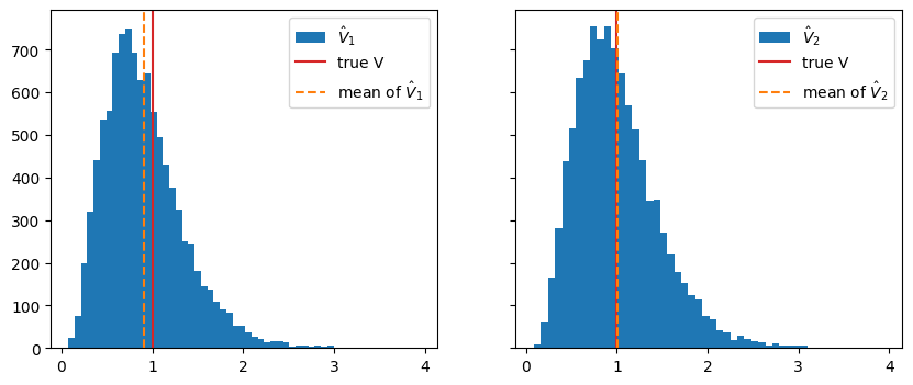

Well-known bias correction for this case: \[ \hat V_{1,\text{corr}} = \frac N{N-1}\hat V_1 \] For derivation see e.g. F. James book (references at end)

Exercise * Compute \(\hat V_{1, \text{corr}}\) and compare its mean with true \(V\)

# do exercise here

# solution

var_1_corr = np.multiply(var_1, N / (N - 1))

print(f"<hat V_1>            = {np.mean(var_1):.2f}")
print(f"<hat V_1(corrected)> = {np.mean(var_1_corr):.2f}")
print(f"truth                = {sigma**2:.2f}")

<hat V_1>            = 0.91
<hat V_1(corrected)> = 1.01
truth                = 1.00

Plug-in estimator

Plug-in principle: replace true values in some formula with estimates, e.g.

\[ c = g(a, b, \dots) \to \hat c = g(\hat a, \hat b, \dots) \]

Justification
- For \(N\to \infty\), \(\Delta a = \hat a - a \to 0\) for any reasonable estimator
- \(g(\hat a) = g(a + \Delta a) = g(a) + O(\Delta a) \to g(a)\) for smooth \(g\)
Example: \(\sqrt{N}\) uncertainty estimator for Poisson-distributed count \(N\)
- \(P(N; \lambda) = e^{-\lambda} \lambda^N / N!\)
- Variance of counts: \(V_N = \lambda\)
- Estimator \(\hat \lambda = \frac 1 K \sum_k N_k\); for \(K = 1\), \(\hat \lambda = N\)
- Plug-in principle: \(\hat V_N = \hat \lambda = N\)
- Standard deviation: \(\hat \sigma_N = \sqrt{\hat V_N} = \sqrt{N}\)
Plug-in estimators can behave poorly in small samples
Poisson example: \(\lambda = 0.01\), sample \(N = 0 \to \hat \sigma_N = 0\)

Bootstrapping bias and variance of estimators

Bootstrap method: generic way to compute bias and variance of any estimator

Parametric bootstrap

Available:
- Sample \(\{ x_i \}\) distributed along \(f(x; a)\), \(a\) is unknown
- Estimator for \(\hat a\)
Want to know bias and variance of estimator
Simulate experiment \(K\) times
- Draw samples \(\{ x_i \}_k\) of equal size from \(\hat f(x; \hat a)\) (plugin-estimate)
- Compute \(\hat a_k\)
- Bias \(\frac 1 K \sum_k (\hat a_k - \hat a)\)
- Variance \(\frac 1 {K-1} \sum_k (\hat a_k - \frac 1K \sum_k \hat a_k)^2\)

from numba_stats import norm, truncexpon, poisson


def make_data(s, mu, sigma, b, slope, seed):
    sr = poisson.rvs(s, size=1, random_state=seed)[0]
    br = poisson.rvs(b, size=1, random_state=seed)[0]
    s = norm.rvs(mu, sigma, size=sr, random_state=seed)
    b = truncexpon.rvs(0, 1, 0, slope, size=br, random_state=seed)
    return np.append(s, b)

truth = {
    "s": 1000,
    "mu": 0.5,
    "sigma": 0.05,
    "b": 500,
    "slope": 1,
}

x = make_data(**truth, seed=0)

w, xe = plt.hist(x, bins=100)[:2];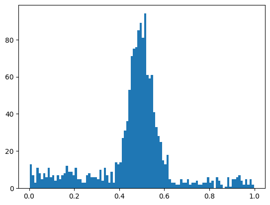

from iminuit import Minuit
from iminuit.cost import ExtendedBinnedNLL
from numba_stats import norm, truncexpon

def model(x, s, mu, sigma, b, slope):
    return s * norm.cdf(x, mu, sigma) + b * truncexpon.cdf(x, 0, 1, 0, slope)

nll = ExtendedBinnedNLL(w, xe, model)
m = Minuit(nll, **truth)
m.limits["mu"] = (0, 1)
m.limits["s", "b", "sigma", "slope"] = (0, None)

m.migrad()

Migrad
FCN = 106.9 (χ²/ndof = 1.1)	Nfcn = 101
EDM = 9.95e-07 (Goal: 0.0002)
Valid Minimum	Below EDM threshold (goal x 10)
No parameters at limit	Below call limit
Hesse ok	Covariance accurate

	Name	Value	Hesse Error	Minos Error-	Minos Error+	Limit-	Limit+	Fixed
0	s	1000	35			0
1	mu	0.4983	0.0018			0	1
2	sigma	0.0482	0.0014			0
3	b	510	27			0
4	slope	0.95	0.15			0

	s	mu	sigma	b	slope
s	1.2e+03	-48.4e-6	8.9237e-3 (0.177)	-0.2e3 (-0.213)	-0.368 (-0.073)
mu	-48.4e-6	3.09e-06	-0 (-0.005)	61.5e-6 (0.001)	-17.0e-6 (-0.066)
sigma	8.9237e-3 (0.177)	-0 (-0.005)	2.12e-06	-8.9641e-3 (-0.231)	-16.5e-6 (-0.078)
b	-0.2e3 (-0.213)	61.5e-6 (0.001)	-8.9641e-3 (-0.231)	711	0.354 (0.091)
slope	-0.368 (-0.073)	-17.0e-6 (-0.066)	-16.5e-6 (-0.078)	0.354 (0.091)	0.0213

Fit can be written as estimator

def estimator(x):
    w = np.histogram(x, bins=xe)[0]
    nll = ExtendedBinnedNLL(w, xe, model)
    m = Minuit(nll, **truth)
    m.limits["mu"] = (0, 1)
    m.limits["s", "b", "sigma", "slope"] = (0, None)
    m.migrad()
    assert m.valid
    return m.values

replicates = []
for seed in range(100):
    x_k = make_data(*m.values, seed=seed+1)
    p_k = estimator(x_k)
    replicates.append(p_k)

replicates = np.transpose(replicates)

Exercise

Compute bias and standard deviation of replicates for each parameter
Compare standard deviation of replicates with Minuit’s uncertainty estimate, accessible via m.errors

# do exercise here

# solution

for i, name in enumerate(m.parameters):
    p = m.values[i]
    r = replicates[i]
    bias = np.mean(r - p)
    std = np.std(r, ddof=1)
    print(f"{name:8} 𝜎(Minuit) = {m.errors[i]:6.2g} 𝜎(bootstrap) = {std:6.2g} "
          f"bias/𝜎 = {bias / std:5.2f}")

s        𝜎(Minuit) =     35 𝜎(bootstrap) =     34 bias/𝜎 = -0.06
mu       𝜎(Minuit) = 0.0018 𝜎(bootstrap) = 0.0017 bias/𝜎 = -0.07
sigma    𝜎(Minuit) = 0.0015 𝜎(bootstrap) = 0.0016 bias/𝜎 = -0.03
b        𝜎(Minuit) =     27 𝜎(bootstrap) =     24 bias/𝜎 = -0.12
slope    𝜎(Minuit) =   0.15 𝜎(bootstrap) =   0.16 bias/𝜎 = -0.09

Nonparametric bootstrap

Can do the same by sampling directly from \(\{ x_i \}\)
Standard method for samples of fixed size \(N\):
- Pick \(N\) random samples from \(\{ x_i \}\) with replacement to obtain \(\{ x_i \}_k\)
- Compute \(\hat a_k\) from \(\{ x_i \}_k\) and proceed as before
“Extended method” for samples of variable size (Poisson):
- Randomly draw \(M\) from Poisson distribution with \(\lambda = N\)
- Pick \(M\) random samples from \(\{ x_i \}\) with replacement to obtain \(\{ x_i \}_k\)
- …
Convenient: use same algorithms for any distribution
Efficient implementations for both algorithms in resample

import resample

resample.__version__

'1.7.1'

from resample.bootstrap import resample

# generate replicated samples of varying size (Poisson distributed)
for x_k in resample(x, size=100, method="extended", random_state=1):
    print(x_k)
    break

[0.58820262 0.58820262 0.52000786 ... 0.38532216 0.26892968 0.26892968]

Exercise

Again compute replicated fit results using resampe and store results in a list
Copy previous code where possible
Again compute bias and standard deviation of replicates and compare with Minuit’s uncertainty estimate

# do exercise here

# solution

replicates = []
for x_k in resample(x, size=100, method="extended", random_state=1):
    replicates.append(estimator(x_k))

replicates = np.transpose(replicates)

for i, name in enumerate(m.parameters):
    p = m.values[i]
    r = replicates[i]
    bias = np.mean(r - p)
    std = np.std(r, ddof=1)
    print(f"{name:8} 𝜎(Minuit) = {m.errors[i]:6.2g} 𝜎(bootstrap) = {std:6.2g}"
          f" bias/𝜎 = {bias / std:5.2f}")

s        𝜎(Minuit) =     35 𝜎(bootstrap) =     33 bias/𝜎 = -0.18
mu       𝜎(Minuit) = 0.0018 𝜎(bootstrap) = 0.0017 bias/𝜎 =  0.10
sigma    𝜎(Minuit) = 0.0015 𝜎(bootstrap) = 0.0014 bias/𝜎 = -0.05
b        𝜎(Minuit) =     27 𝜎(bootstrap) =     27 bias/𝜎 = -0.04
slope    𝜎(Minuit) =   0.15 𝜎(bootstrap) =   0.17 bias/𝜎 =  0.18

resample provides shortcut for computing variance

from resample.bootstrap import variance

var = variance(estimator, x, method="extended", size=100, random_state=1)

for i, name in enumerate(m.parameters):
    std = var[i] ** 0.5
    print(f"{name:8} 𝜎(Minuit) = {m.errors[i]:6.2g} 𝜎(bootstrap) = {std:6.2g}")

s        𝜎(Minuit) =     35 𝜎(bootstrap) =     33
mu       𝜎(Minuit) = 0.0018 𝜎(bootstrap) = 0.0017
sigma    𝜎(Minuit) = 0.0015 𝜎(bootstrap) = 0.0014
b        𝜎(Minuit) =     27 𝜎(bootstrap) =     27
slope    𝜎(Minuit) =   0.15 𝜎(bootstrap) =   0.17

Exercise

Repeat the variance calculation without using method="extended"
Compare the uncertainties of \(s\) and \(b\)

# do exercise here

# solution

var2 = variance(estimator, x, size=100, random_state=1)

# uncertainties of s and b are too small, if normal bootstrap is used,
# since size variation is not simulated
for i, name in enumerate(m.parameters):
    std = var[i] ** 0.5
    std2 = var2[i] ** 0.5
    print(f"{name:8} 𝜎(extended bootstrap) = {std:6.2g} "
          f"𝜎(normal bootstrap) = {std2:6.2g}")

s        𝜎(extended bootstrap) =     33 𝜎(normal bootstrap) =     24
mu       𝜎(extended bootstrap) = 0.0017 𝜎(normal bootstrap) = 0.0018
sigma    𝜎(extended bootstrap) = 0.0014 𝜎(normal bootstrap) = 0.0016
b        𝜎(extended bootstrap) =     27 𝜎(normal bootstrap) =     24
slope    𝜎(extended bootstrap) =   0.17 𝜎(normal bootstrap) =   0.17

Bootstrap can be applied to most statistical problems in HEP
Restriction: samples must be identically and independently distributed
May work well even with small samples (< 10)

Error propagation

Full analysis typically combines many intermediate results with uncertainties into final result
Consider \(\vec b = g(\vec a)\) with uncertainties in \(\vec a\)
Two ways of computing uncertainties of \(\vec b\)
- Monte-Carlo simulation
- Error propagation
Can be equally used for statistical and systematic uncertainties

Monte-Carlo simulation

Draw variations of fit result from multivariate normal distribution
Compute variable of interest from variations
Compute standard deviation or covariance of
Example: compute uncertainty of \(\hat N = \hat s + \hat b\)

rng = np.random.default_rng(1)
a_k = rng.multivariate_normal(m.values, m.covariance, size=1000)

def g(a):
    return a[0] + a[3]

b_k = np.apply_along_axis(g, -1, a_k)

print(f"𝜎(N, simulation) = {np.std(b_k):.3g}")
print(f"𝜎(N, naive)      = {(m.errors[0]**2 + m.errors[3]**2)**0.5:.3g}")
print(f"𝜎(N, expected)   = {np.sqrt(len(x)):.3g}")

𝜎(N, simulation) = 37.7
𝜎(N, naive)      = 43.7
𝜎(N, expected)   = 38.8

\(\sigma_{N,\text{simulation}}^2 < \sigma_s^2 + \sigma_b^2\), because \(s_k\) and \(b_k\) are anti-correlated

Error propagation

Given: \(\vec a\) with covariance matrix \(C_a\) and differentiable function \(\vec b = g(\vec a)\)
\(\vec b\) can have different dimensionality from \(\vec a\)
One can derive via first-order Taylor expansion: \[ C_b = J \, C_a \, J^T \text{ with } J_{ik} = \frac{\partial g_i}{\partial a_k} \]
Useful special cases
- Sum of scaled independent random values \(c = \alpha a + \beta b\) (\(\alpha, \beta\) are constant) \[ \sigma^2_c = \alpha^2 \sigma^2_a + \beta^2 \sigma^2_b \]
- Product of powers of independent random values \(c = a^\alpha \, b^\beta\) \[ \left(\frac{\sigma_c}{c}\right)^2 = \alpha^2 \left(\frac{\sigma_a}{a}\right)^2 + \beta^2 \left(\frac{\sigma_b}{b}\right)^2 \]
Final uncertainty often dominated by one term
When estimating systematic uncertainties: put your effort in estimating largest term and be lax on others
Computation of \(J\) by hand error-prone and tedious
jacobi library offers automatic error propagation based on a robust numerical derivative

import jacobi

jacobi.__version__

'0.9.2'

b, cov_b = jacobi.propagate(g, m.values, m.covariance)

f"𝜎(N, error propagation) = {cov_b ** 0.5:.3g} 𝜎(N, expected) = {np.sqrt(len(x)):.3g}"

'𝜎(N, error propagation) = 38.9 𝜎(N, expected) = 38.8'

jacobi.propagate works for any differentiable mapping, which even includes most fits!

from iminuit.cost import LeastSquares

def h(pvec):
    rng = np.random.default_rng(1)
    a, b = pvec
    x = np.array([1, 2, 3])
    y = rng.normal(a + b * x, 0.1)
    m = Minuit(LeastSquares(x, y, 0.1, lambda x, a, b: a + b * x), a=0, b=0)
    m.strategy = 0
    m.migrad()
    assert m.valid
    return m.values

jacobi.propagate(h, (1, 2), (1, 1))

(array([1.05143603, 1.99924264]),
 array([[1.00000000e+00, 1.44351198e-12],
        [1.44351198e-12, 1.00000000e+00]]))

Systematic uncertainties: Known unknowns

“There are known knowns, things we know that we know;
and there are known unknowns, things that we know we don’t know.
But there are also unknown unknowns, things we do not know we don’t know.”
Donald Rumsfeld

Why data analyses take so long: study data, detector, and methods to turn unknown unknowns into known knowns or known unknowns
known unknowns = systematic uncertainties
No formal way, but generally…

Worry * What could go wrong? * What are my assumptions?

Example * Efficiency or correction factor taken from simulation, but simulation differs from real experiment * Solution: perform control measurement to estimate how much simulation differs from real experiment

Methods * Use methods that are known to be optimal for your problem or derive them from first principles * General purpose methods often safer to use than special-case methods * Maximum-likelihood fit > least-squares fit * Bootstrap estimate of uncertainty > other uncertainty estimates

Apply checks * Validate whole analysis on simulated data (sometimes you can use toy simulation) * Split data by magnet polarity, fill, etc., analyze splits separately, check for agreement

Guidelines for handling systematic errors * Roger Barlow: Systematic Errors: Facts and Fictions (2002) * Roger Barlow, “Practical Statistics for Particle Physics” (2019), Section 6.5

Further resources for learning

LHCb Statistics and ML WG

TWiki page
Statistics Guidelines to collect information about best practices

Introductory statistics books

List of books on TWiki pages of Statistis and Machine Learning WG
Books I personally like a lot
- Glen Cowan, “Statistical Data Analysis”, Oxford University Press, 1998
- F. James, “Statistical Methods in Experimental Physics”, 2nd edition, World Scientific, 2006
- R. Barlow, “Statistics: a Guide to the Use of Statistical Methods in the Physical Sciences”, Wiley, 1989
- B. Efron, R.J. Tibshirani, “An Introduction to the Bootstrap”, CRC Press, 1994

Lectures, papers, notebooks

Roger Barlow
More Jupyter notebooks
All about sWeights and COWs with gentle derivation
- HD, M. Kenzie, C. Langenbruch, M. Schmelling, Nucl.Instrum.Meth.A 1040 (2022) 167270