Introduction into Machine Learning

Hans Dembinski

Overview

• Caution: Field is riddled with buzzwords

  • Machine learning, artificial intelligence, deep learning, belief networks, attention-based networks, long short-term memory, features, hyperparameters …

• Anthropomorphized and technical names hide what are usually basic mathematical algorithms

• Machine learning: umbrella term for multivariate statistical methods for classification and regression

  • Multivariate: algorithms use more than one variable as input, e.g. (x, y, z)
  • Statistical: algorithms can handle noisy input and are founded on statistical theory
  • Classification: sort inputs based on input variables into categories
  • Regression: find a mapping of input vectors to output vectors (fitting)

• Rise of the machines: Why do we need them?
  • Humans good at working with 1D or 2D data, because we can visualize it
  • Humans bad at working with higer-dimensional data
  • Algorithms (“machines”) scale well to high-dimensional data

Notable software

• Multiple algorithms and utilities
  • Scikit-Learn
  • ROOT TMVA
• Gradient-boosted decision trees (aka gradient boosting machines)
  • XGBoost
  • LightGBM
  • CatBoost
  • …
• Neural networks
  • Tensorflow
  • Keras (high-level interface to Tensorflow)
  • PyTorch
  • …

Learning resources

• Internet provides excellent resources for autodidactic learning

  • Example code
  • Tutorials
  • Documentation
    
    

• Scikit-Learn

• Kaggle

• All methods can do classification and regression and work with any input

• What to use?

  • Structured data (i.e. tables of numbers): Ensembles of decision trees
    • Good results with default settings
    • Can process continuous and categorical input (m/w, red/green/blue, …)
    • No data preprocessing required
    • Compute feature importance
  • Unstructured data (i.e. images, waveforms, text…): Neural networks
    • Deep networks learn to extract features automatically
    • Requires data preprocessing
    • Networks difficult to optimize for non-experts
    • Often need very large data sets for training

Some definitions * sample: one or more numbers which describe outcome of stochastic process * dataset: consists of samples * features: subset of numbers from each sample which carry interesting information, also numbers computed from each sample * signal: samples which originate from stochastic process of interest, typically particle decay * background: samples which do not originate from process of interest

Discuss how the typical decay \(K^0_S \to \pi^+ \pi^-\) is reconstructed and why in general there is always some background.

Clarify how the previous terms would be used in the context of this example.

Classification

• Setting: dataset is mix of two or more components, typically signal + one or more backgrounds
• Want only signal component, invert a cut to select signal candidates
• Features are variables which allow to discriminate between signal and background, for example, reconstructed mass of decay candidate

#!pip install scipy matplotlib numpy scikit-learn xgboost

import scipy
import matplotlib
import numpy
import sklearn
import xgboost

print(f"scipy {scipy.__version__}")
print(f"matplotlib {matplotlib.__version__}")
print(f"numpy {numpy.__version__}")
print(f"sklearn {sklearn.__version__}")
print(f"xgboost {xgboost.__version__}")

scipy 1.10.0
matplotlib 3.7.1
numpy 1.21.6
sklearn 1.2.2
xgboost 1.7.4

from scipy.stats import norm
from matplotlib import pyplot as plt
import numpy as np

background = norm(0, 1).rvs(1000, random_state=1)
signal = norm(1, 0.1).rvs(500, random_state=1)

x = np.append(signal, background)
y = np.append(np.ones(len(signal)), np.zeros(len(background)))

def plot(x, y):
    signal = x[y == 1]
    background = x[y == 0]
    t, xe = np.histogram(x, bins=100)
    s = np.histogram(signal, bins=xe)[0]
    b = np.histogram(background, bins=xe)[0]
    plt.stairs(b, xe, fill=True, label="background")
    plt.stairs(t, xe, baseline=b, fill=True, label="signal")
    plt.xlabel("x")
    plt.legend();
    return xe

plot(x, y);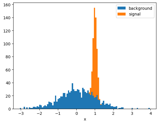

Exercise: * Propose simple selection (“cut”) that keeps most of the signal and removes most of the background * Is it possible to eliminate the background completely?

Efficiency and purity of a selection

• Efficiency: fraction of signal left after applying selection
  • Number of true signal samples after cut / Number of all true signal samples
• Purity: fraction of background still contained in selected sample
  • Number of true signal samples after cut / Number of selected samples
• Want to maximize efficiency and purity

Single-parameter cut

xmin = 0.7

selected_signal = np.sum(x[y==1] > xmin)
total_signal = np.sum(y==1)
selected = np.sum(x > xmin)

efficiency = selected_signal / total_signal
purity = selected_signal / selected

plot(x, y)
plt.axvspan(-3.5, xmin, facecolor="k", alpha=0.5)
plt.legend(title=f"efficiency={efficiency:.2f}\npurity={purity:.2f}");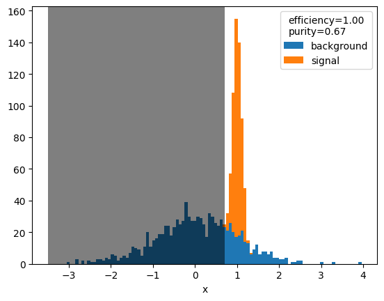

xmin = np.linspace(-3, 3, 100)
efficiency = []
purity = []
for xm in xmin:
    selected_signal = np.sum(signal > xm)
    total_signal = len(signal)
    selected = np.sum(x > xm)
    e = selected_signal / total_signal
    p = selected_signal / selected
    efficiency.append(e)
    purity.append(p)
plt.plot(xmin, efficiency, label="efficiency")
plt.plot(xmin, purity, label="purity")
plt.xlabel("xmin")
plt.legend();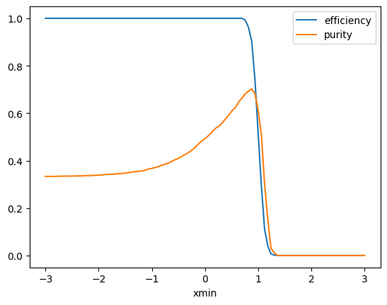

plt.scatter(efficiency, purity, c=xmin);
plt.xlim(0, 1)
plt.ylim(0, 1)
plt.xlabel("efficiency")
plt.ylabel("purity")
plt.colorbar().set_label("xmin")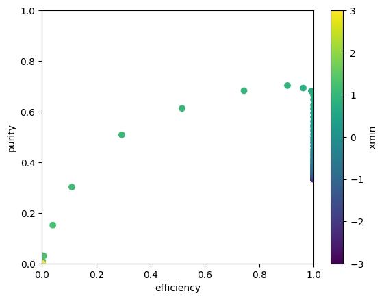

arg = np.argmax(purity)
print("efficiency at max purity", efficiency[arg])

efficiency at max purity 0.904

• How to choose cut?

  • Want to maximize efficiency and purity, but what trade-off between the two?

• Often subjective choice is acceptable, because exact answer is difficult

• Objective answer given by figure-of-merit (FOM)

  • Popular is Punzi FOM
  • Most FOM (including Punzi FOM) only minimize statistical uncertainty
  • Correct FOM has to minimize total uncertainty = statistical ⊕ systematic
  • Systematic uncertainty often difficult to quantify: fallback to Punzi or subjective choice

BDT-based cut

• We can do better with two cuts, on xmin and xmax

• Space of cut parameters then already two-dimensional

• With 2D data

  • Four rectangular cuts possible (4 cut parameters)
  • Infinitely many non-rectangular cuts possible

• Use machine instead, needs to be trained on labeled data

• Use BDT classifier from XGBoost

• Gradient boosting machines regularly win Kaggle competitions

• Well documented, fast, parallizable, tunable

from xgboost.sklearn import XGBClassifier
from sklearn.model_selection import train_test_split

# generate training data, ideally we have more than actual data
background = norm(0, 1).rvs(100000, random_state=2)
signal = norm(1, 0.1).rvs(50000, random_state=2)
x2 = np.append(signal, background)

# features in general matrix [N, K] for N samples and K features
X = x2.reshape((len(x2), 1))
# labels: signal=1, background=0
y = np.append(np.ones_like(signal), np.zeros_like(background))

# ALWAYS do this: split into train and test datasets
X_train, X_test, y_train, y_test = train_test_split(X, y, random_state=3)

# actual magic happens here
clf = XGBClassifier(random_state=4)
clf.fit(X_train, y_train);

fig, ax = plt.subplots(2, sharex=True)

plt.sca(ax[0])
xe = plot(X_test[:, 0], y_test)
plt.xlabel(None)  # unset label set by `plot`

plt.sca(ax[1])
score = clf.score(X_test, y_test)
xm = np.linspace(xe[0], xe[-1], 200)
ps, pb = clf.predict_proba(xm).T

plt.xlabel("x")
plt.plot(xm, ps, "C0-", label="background probability")
plt.plot(xm, pb, "C1-", label="signal probability")
plt.legend(title=f"score={score:.2f}", frameon=False);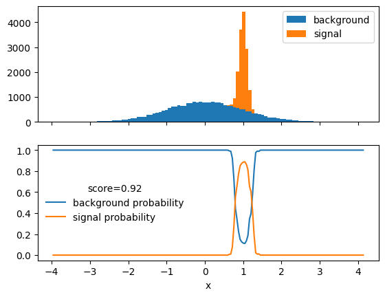

Exercise: * Vary some hyperparameters in XGBClassifier to see how score, runtime, and predicted probability changes * n_estimators try e.g. 2, 5, 10 * max_depth try e.g. 1, 5, 10 * learning_rate try e.g. 0.001, 0.05, 0.5, 1

• BDT predicts signal probability
• We use this to implement our cut: select regions with high signal probability

ps = clf.predict_proba(X_test[y_test==1])[:, 1]
pb = clf.predict_proba(X_test[y_test==0])[:, 1]
xe = plt.hist(ps, bins=20, alpha=0.5, label="true signal")[1]
plt.hist(pb, bins=xe, alpha=0.5, label="true background")
plt.legend()
plt.xlabel("predicted signal probability")
plt.ylim(0, 5e3);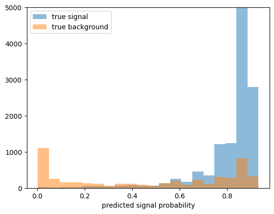

xe = plot(X_test[:, 0], y_test)

# chosen cut: signal probability > 0.6
# visualize accepted region
xm = np.linspace(xe[0], xe[-1], 200)
mask = clf.predict_proba(xm)[:, 1] > 0.6
plt.plot(xm, mask * 5000, "k-");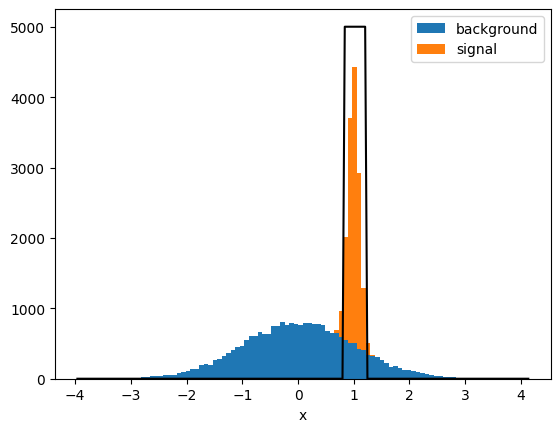

pmin = np.linspace(0, 1, 100)
efficiency = []
purity = []
for pm in pmin:
    mask = clf.predict_proba(X_test)[:, 1] > pm
    selected = np.sum(mask)
    selected_signal = np.sum(y_test[mask])
    total_signal = np.sum(y_test)
    efficiency.append(selected_signal / total_signal)
    with np.errstate(divide="ignore", invalid="ignore"):
        purity.append(selected_signal / selected)
plt.plot(pmin, efficiency, label="efficiency")
plt.plot(pmin, purity, label="purity")
plt.xlabel("pmin")
plt.legend();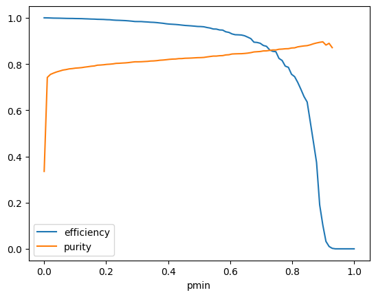

plt.scatter(efficiency, purity, c=pmin);
plt.xlim(0, 1)
plt.ylim(0, 1)
plt.xlabel("efficiency")
plt.ylabel("purity")
plt.colorbar().set_label("pmin")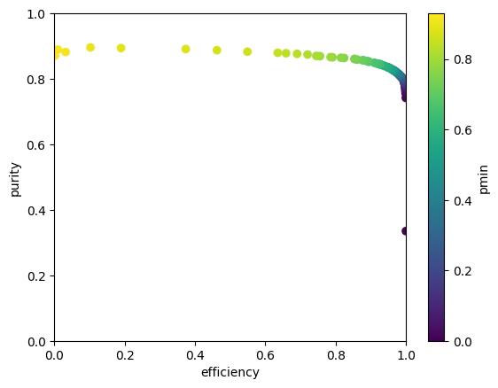

• Physicists like efficiency and purity, but ROC curve is standard
• Receiver-operator characteristic
• ROC plots true positive rate (fraction of signal that passes cut) over false positive rate (fraction of background that passes cut)
• Scikit-Learn provides a quick way to generate this plot

from sklearn.metrics import RocCurveDisplay

RocCurveDisplay.from_estimator(clf, X_test, y_test);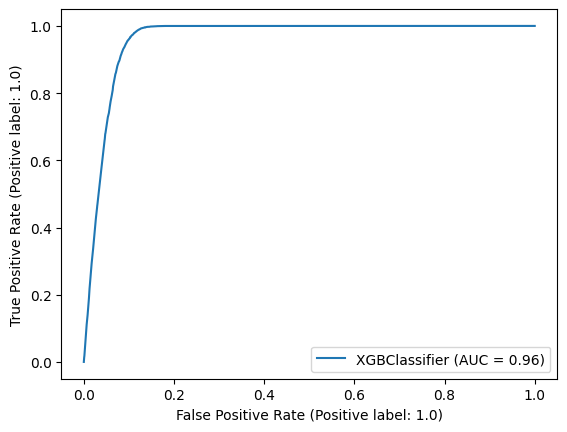

• area under curve (AUC) is a common metric to compare the performance of two different classifiers
• can also use Scikit-Learn to compute ROC points and AUC and plot these ourselves

from sklearn.metrics import roc_curve, auc

# plot XGBoost curve again
fpr, tpr, thresholds = roc_curve(y_test, clf.predict_proba(X_test)[:, 1])
plt.plot(fpr, tpr, label=f"XGBoost AUC={auc(fpr, tpr):.2f}")

# plot ROC curve for our simple x > 0.7 cut for comparison
fpr2, tpr2, _ = roc_curve(y_test, X_test[:, 0] > 0.7)
plt.plot(fpr2, tpr2, label=f"x > 0.7 AUC={auc(fpr2, tpr2):.2f}")

plt.xlabel("False positive rate")
plt.ylabel("True positive rate")
plt.legend();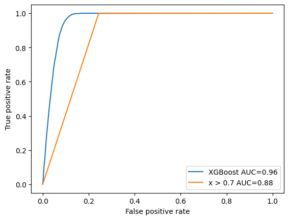

• Exercise: run scikit-learn example
• Try adding XGBClassifier into the comparison
• Play around with the hyperparameters of the classifiers

Regression

• Regression (aka fitting): “learn” function y = f(x) from points(x, y), where both x and y can be vectors

• Machines can do this, but we rarely need this in HEP

• We usually prefer to use theoretically motivated models or hand-crafted low-order polynoms

• Let’s try regression on one-dimensional function

def model(x, a, b, c, d):
    return a + b * np.sin(c * x) * np.exp(- d * x)

truth = 0.2, 1, 2, 0.5

x = np.linspace(0, 10, 1000)
plt.plot(x, model(x, *truth))
plt.xlabel("x")
plt.ylabel("y");

• generate random points on this curve and add some noise to make it more realistic

rng = np.random.default_rng(1)

x = rng.uniform(0, 10, 1000)
y = model(x, 0.2, 1, 2, 0.5)
y += rng.normal(0, 0.05, len(y))

X = np.reshape(x, (-1, 1))

• (X, y) are inputs for regression similar to before, but y is a real number now, not a label (integer)

Neural network

• We use MLPRegressor from Scikit-Learn, a basic neural network
• Neural networks always need preprocessing
• Scikit-Learn offers pipelines to automate this, use them

from sklearn.neural_network import MLPRegressor
from sklearn.preprocessing import StandardScaler
from sklearn.pipeline import make_pipeline

# network with 5 hidden layers with 100 nodes each
regressor = MLPRegressor(
    hidden_layer_sizes=(100,)*5,
    random_state=1)

# we use basic StandardScaler for preprocessing
pipeline = make_pipeline(StandardScaler(), regressor)
pipeline.fit(X, y);

# compute fitted curve
X2 = np.reshape(np.linspace(0, 10, 1000), (-1, 1))
y2 = pipeline.predict(X2)

plt.plot(x, y, ".")
plt.plot(X2[:, 0], y2, color="r", label="Neural net")
plt.plot(X2[:, 0], model(X2[:, 0], *truth), color="k", label="truth")
plt.legend()
plt.xlabel("x")
plt.ylabel("y");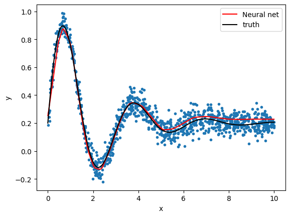

• Exercise: play around with hyperparameters of MLPRegressor
• What happens if you remove the StandardScaler?
• What performs better, deep or wide networks?

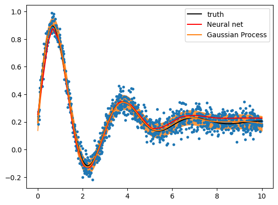
Gaussian Process

• For low-dimensional data, Gaussian Process Regression can work well
• Not easy to set up: need to select suitable kernels and configure them
• Advantage: Predicts uncertainty and automatically provides smooth solution

from sklearn.gaussian_process import GaussianProcessRegressor
from sklearn.gaussian_process.kernels import RBF, WhiteKernel

kernel = RBF() + WhiteKernel()

gpr = GaussianProcessRegressor(kernel=kernel)
gpr.fit(X, y)
y3, y3err = gpr.predict(X2, return_std=True)

plt.plot(x, y, ".")
plt.plot(X2[:, 0], model(X2[:, 0], *truth), color="k", label="truth")
plt.plot(X2[:, 0], y2, color="r", label="Neural net")
l = plt.plot(X2[:, 0], y3, label="Gaussian Process")[0]
plt.fill_between(X2[:, 0], y3 - y3err, y3 + y3err, alpha=0.8, color=l.get_color())
plt.legend();