# Example: standard normal distribution ("Gaussian")
from matplotlib import pyplot as plt
import numpy as np
from scipy.stats import norm
x = np.linspace(-5, 5, 1000)
fx = norm.pdf(x)
Fx = norm.cdf(x)
sample = norm.rvs(size=50, random_state=1)by Hans Dembinski, TU Dortmund
What is an uncertainty, really?
We write \(a = 3 \pm 0.5\), where 0.5 is the standard error (jargon: “error” = uncertainty).
What does this truely mean?
The true value given by nature is 3, but when we measure it, it fluctuates (e.g. Heisenberg uncertainty principle).
I made an experiment and this expresses my belief that the value is most likely 3 and is located within the interval 2.5 to 3.5 with 68 % probability. This is based on the data that I recorded and my initial assumption that the value of \(a\) is positive.
Someone made an experiment and their estimate for the true value of \(a\) based on the data is 3. The interval (2.5, 3.5) contains the true value with 68 % probability.
- Is nonsense, but b) and c) are valid interpretations
- In HEP, we generally mean c), because we compute uncertainties based on the Frequentist school of statistics
- follows from the Bayesian school of statistics
- In b) or c), what does “68% probability” really mean in each context?
Statistical and systematic uncertainties
- Either type can be correlated or uncorrelated
Statistical uncertainty
Origin: We use finite sample instead of infinite distribution
Goes down as simple size increases
Example
- Arithmetic mean \(\bar x = \frac 1N\sum_i x_i\)
- Variance of mean $ = {N(N - 1)}_i (x_i - x)^2$
We have reliable standard recipes to calculate these
Variance or standard deviation?
- Standard deviation \(\sigma = \sqrt{V}\)
- We communicate standard deviations, but compute variances
- Variance is more fundamental
- Second central moment of distribution
- \(V = V_1 + V_2\), but \(\sigma = \sqrt{\sigma_1^2 + \sigma_2^2}\)
Systematic uncertainty
- Origin: Imperfect appartus or technique, deviations of reality from simplified models
- Quantifies potential mistakes in analysis or lack of knowledge
- Does not go down as sample size increases
- Correlated examples
- Real-life: Measured the length of ten shoes with ruler than has factory tolerance of 0.1 mm
- LHCb: Measured cross-sections with value of luminosity that has uncertainty of 1-2%
- Uncorrelated examples
- Real-life: ???
- LHCb: Measured momentum of particle in LHCb differs from true momentum \(\sigma_p/p \approx 0.5\!-\!1\%\)
- Conceptually different, requires different math
- Not well covered in statistics books, but some theoretical results available
- Many misconceptions
Statistical errors can be systematic errors
- Depends on context
- Statistical error of parameter in control study is systematic error in main study
- Example: LHCb performs calibration measurements to determine tracking and PID efficiencies
- Statistical errors in calibration measurements are systematic errors in main measurement
Statistical uncertainties: Basic concepts
We need to distinguish between true value, estimator, and estimate (or estimated value).
- Sample \(\{ x_i \}\) drawn from distribution \(F(x)\) consists of random values \(x_i\) that are independent and identically distributed (iid)
- Sample values occur with probability
- \(P(k) = F(k)\) if \(k\) discrete
- \(d P(x) = d F(x) = f(x) dx\) if \(x\) continuous
- \(f(x)\) probability density function (pdf)
- \(F(x)\) cumulative density function (cdf)
- Will refer to \(f(x)\) and \(F(x)\) as the distribution
- Beware lax jargon: distribution != sample
plot()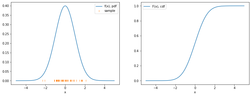
- Distribution usually depends on parameters that we are interested in
- Example: Normal distribution depends on parameters \(\mu, \sigma\) (location, width)
- Notation: \(f(x; a, b, \dots)\), semicolon separates random variable \(x\) from parameters \(a, b, \dots\)
- In general, \(x\) can be a vector and parameters can be written as vector, too: \(f(\vec x; \vec a)\)
Estimation
- Estimation is statistician speak for “measurement”
- We have sample \(\{ x_i \}\) which is distributed according to \(f(x; a)\), \(a\) is unknown
- Estimator \(h[x]\) maps data sample to estimate \(\hat a\) of \(a\)
- Notation
- \(h[x]\) estimator maps sample \(\{ x_i \}\) to value
- \(f(x)\) is function that maps value to value
- Examples of estimators of location of distribution
- Arithmetic mean \(h_1[x] = \frac 1N \sum_i x_i\)
- Sample median \(h_2[x]\): Sort \(x_i\), pick value in the middle
- Estimator can be formula in closed form or an algorithm (recipe)
# Example: normal distribution with true value mu=1, sigma=0.5
# mu is of interest; sigma is not of interest, a nuisance parameter

from matplotlib import pyplot as plt
import numpy as np
from scipy.stats import norm

mu, sigma = 1, 0.5
dist = norm(mu, sigma)
x = np.linspace(-1, 3, 1000)
sample = dist.rvs(size=20, random_state=1)

est1 = np.mean(sample)
est2 = np.median(sample)
def plot():
plt.plot(x, dist.pdf(x))
plt.xlabel("x")
plt.plot(sample, np.zeros_like(sample), "|")
plt.axvline(dist.stats()[0], label="$\mu$", color="C3")
plt.axvline(est1, ls="--", label="mean", color="C2")
plt.axvline(est2, ls=":", label="median", color="C4")
plt.legend();plot()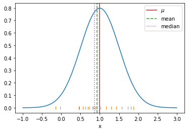
Optimal estimators
- Many kinds of estimators, some better than others
- We want optimal estimators
- Some desirable properties
- As close to true value as possible (we come back to that)
- Easy to compute and/or easy to apply to any problem
- Robustness against outliers
- In HEP, we mainly use
- Maximum-likelihood estimator (MLE)
- Plug-in estimator
- Bootstrap estimator (meta estimator)
How far away is estimate from true value?
- Depends on estimator, sample size, distribution
- Almost magic: accuracy of estimator can be also estimated from sample!
- Define “close to true value”
- In experiment, we have sample \(\{ x_i \}\) with size \(N\) and obtained estimate \(\hat a = h[x]\)
- Sample \(\{ x_i \}\) is random and so is estimate \(\hat a\)
- If experiment is identically repeated \(K\) times, we get sample \(\{ x_i \}_k\) and estimate \(\hat a_k\) each time
- Quantify properties of sample of estimates \(\{ \hat a_1, \hat a_2, \dots, \hat a_K \}\) to describe accuracy of estimator with bias and variance estimates
- Bias: \(\hat B[\hat a] = \frac1K \sum_i (\hat a_i - a)\)
- Variance: \(\hat V[\hat a] = \frac1K\sum_i (\hat a_i - a)^2\)
- Example for a biased estimator: if true mean \(\mu\) is unknown, variance estimate \(\hat V[x] = \frac1N\sum_i (x_i - \hat\mu)^2\) is biased
from matplotlib import pyplot as plt
import numpy as np
from scipy.stats import norm

# true values and distribution
mu, sigma = 1, 1
dist = norm(mu, sigma)

N, K = 10, 1000
var_1, var_2 = [], []
for k in range(K):
    sample = dist.rvs(size=N, random_state=k+1)
    hat_mu = np.mean(sample)
    v1 = np.mean((sample - np.mean(sample)) ** 2)
    v2 = np.mean((sample - mu) ** 2)
    var_1.append(v1)
    var_2.append(v2)
# hidden plotting code used in next cell
def plot():
mu, sigma = dist.stats()
fig, ax = plt.subplots(1, 2, sharex=True, sharey=True, figsize=(14, 5))
ax[0].hist(var_1, bins=50, label="$\hat V[x; \hat \mu]$");
ax[1].hist(var_2, bins=50, label="$\hat V[x; \mu]$");
for axi in ax:
axi.axvline(sigma ** 2, color="C3", label="true V[x]")
ax[0].axvline(np.mean(var_1), color="C1", ls="--", label="mean of $\hat V[x; \hat \mu]$")
ax[1].axvline(np.mean(var_2), color="C1", ls="--", label="mean of $\hat V[x; \mu]$")
for axi in ax:
axi.legend()plot()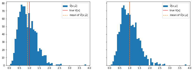
- Perhaps surprising that \(\hat V[x; \hat \mu]\) is biased although \(\hat \mu\) is an unbiased estimate of \(\mu\)
- In this case, simple well-known bias correction: \(\frac N{N-1}\hat V[x; \hat \mu]\) is unbiased (for derivation see e.g. F. James book (references at end))
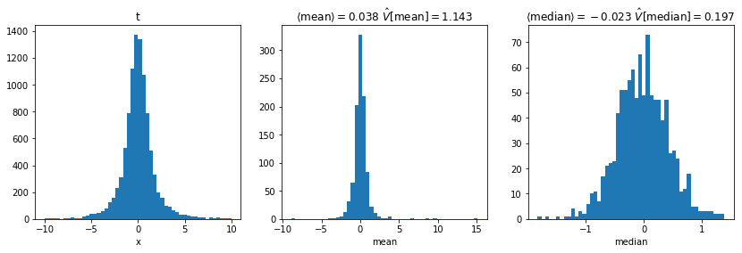
# Example for variance of estimator: variance of mean and median
from matplotlib import pyplot as plt
import numpy as np
from scipy.stats import norm, t

mu, sigma = 0, 1

dist = {
    "norm": norm(mu, sigma),
    "t": t(2, mu, sigma),
}

N, K = 10, 1000
data = {}
for dkey, d in dist.items():
    est = {"mean": [], "median": []}
    all_samples = []
    for k in range(K):
        sample = d.rvs(size=N, random_state=k+1)
        est["mean"].append(np.mean(sample))
        est["median"].append(np.median(sample))
        all_samples.append(sample)
    data[dkey] = est, all_samples
def plot():
for dkey, (est, all_samples) in data.items():
fig, ax = plt.subplots(1, 3, figsize=(14, 4))
ax[0].hist(np.concatenate(all_samples), bins=50, range=(-10, 10))
ax[0].set_title(dkey)
ax[0].set_xlabel("x")
for axi, (key, esti) in zip(ax[1:], est.items()):
axi.hist(esti, bins=50)
axi.set_title(f"$\\langle \mathrm{{{key}}} "
f"\\rangle = {np.mean(esti):.3f}$ "
f"$\hat V[\mathrm{{{key}}}] = {np.var(esti):.3f}$""")
axi.set_xlabel(f"{key}")plot()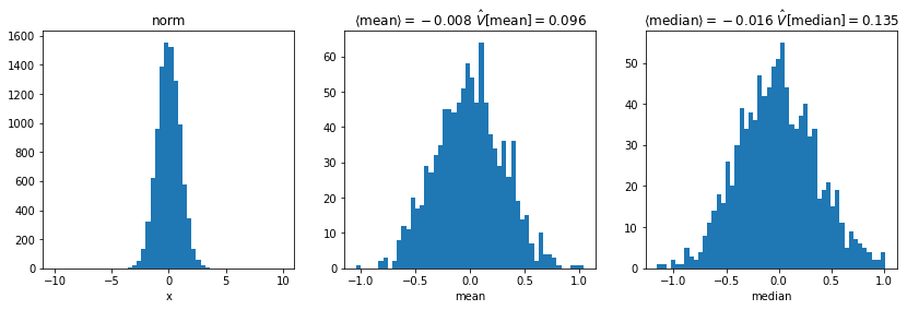
- For normal distribution
- Median has larger variance than arithmetic mean
- For Student’s t distribution
- Median has smaller variance than arithmetic mean
- Which estimator is least biased and has smallest variance depends on distribution
- Good estimator for any distribution: maximum-likelihood estimator
Plug-in estimator
- Plug-in principle: replace true values in some formula with estimates, e.g.
\[ c = g(a, b, \dots) \to \hat c = g(\hat a, \hat b, \dots) \]
- Justification (1D, likewise for ND)
- For \(N\to \infty\), \(\Delta a = \hat a - a \to 0\) for any reasonable estimator
- \(g(\hat a) = g(a + \Delta a) = g(a) + O(\Delta a) \to g(a)\) for smooth \(g\)
- Example: \(\sqrt{N}\) uncertainty estimator for Poisson-distributed count \(N\)
- Variance of Poisson distribution of counts \(N\): \(V_N = \lambda\)
- Plug-in principle: Replace expected count \(\lambda\) with observed count \(N\): \(\hat V_N = N\)
- Standard deviation is square-root of variance: \(\hat \sigma_N = \sqrt{\hat V_N} = \sqrt{N}\)
- Plug-in estimators are usually biased (unless g is linear) and may fail to give reasonable answers for very small samples
- Extreme case: \(\lambda = 0.01\), sample \(N = 0 \to \sqrt{0} = 0 \neq 0.1\)
- Be aware of potentially bias when you use plug-in estimator
Bootstrapping estimator bias and variance
- Bootstrap method is generic way to compute bias and variance of any estimator
- Looks like a magic trick, but well-founded in theory (excellent introductory book by inventor Brad Efron at the end)
Parametric bootstrap
- LHCb jargon: “running toy simulations”
- Situation:
- You have sample \(\{ x_i \}\) distributed along \(f(x; a)\) with unknown parameter \(a\)
- You have estimator \(\hat a = h[x]\) (can be a formula, fit, anything)
- You want to estimate bias and variance of \(h[x]\)
- If we knew true \(a\), could simply simulate the experiment many times
- Generate sample \(\{ x_i \}_k\) from \(f(x; a)\) with same size as \(\{ x_i \}\), compute \(\hat a_k\)
- Compute bias and variance estimates from sample \(\{ \hat a_k \}\) as shown before
- Don’t know \(f(x; a)\), but its plug-in estimate \(\hat f(x) = f(x; \hat a)\)!
- So do the same but sample from \(\hat f(x)\)
- This actually works, and very well!
# parametric bootstrap to estimate variance of mean
import numpy as np
from scipy.stats import norm

mu, sigma = 1, 1
N = 10
sample = norm(mu, sigma).rvs(N, random_state=1)

# in general, we use a fit here to get parameters of distribution
mu_est = np.mean(sample)
sigma_est = np.std(sample, ddof=1)
dist = norm(mu_est, sigma_est)

mu_est_b = []
for k in range(1000):
    b = dist.rvs(N, random_state=k)
    mu_est_b.append(np.mean(b))

print(f"Bias = {np.mean(mu_est_b) - mu_est:.2f} "
      f"std.dev. = {np.std(mu_est_b, ddof=1):.2f} "
      f"(expected: {sigma / N ** 0.5:.2f})")
Bias = -0.01 std.dev. = 0.39 (expected: 0.32)Non-parametric bootstrap
- Taking previous idea one step further
- Sampling does not require \(\hat f(x)\), but \(\hat F(x)\) (the cdf)
- \(\hat F(x)\) can be estimated directly from sample \(\{ x_i \}\) (empirical cdf)
- Accuracy a bit worse than parametric bootstrap, but even easier to use
# bootstrap bias and variance of arithmetic mean
import numpy as np
from resample.bootstrap import resample
from scipy.stats import norm

mu, sigma = 1, 1
N = 10
sample = norm(mu, sigma).rvs(N, random_state=1)

mu_est_b = []
for replicas in resample(sample, size=1000):
    mu_est_b.append(np.mean(replicas))

print(f"Bias = {np.mean(mu_est_b) - mu_est:.2f} "
      f"std.dev. = {np.std(mu_est_b, ddof=1):.2f} "
      f"(expected: {sigma / N ** 0.5:.2f})")
Bias = 0.00 std.dev. = 0.38 (expected: 0.32)# Bonus: bootstrap bias and variance of np.var
import numpy as np
from resample.bootstrap import bias, variance
from scipy.stats import norm
mu, sigma = 1, 1
N = 10
sample = norm(mu, sigma).rvs(N, random_state=1)
for ddof in (0, 1):
def fn(s):
return np.var(s, ddof=ddof)
print(f"Bias = {bias(fn, sample, random_state=1):.2f} "
f"std.dev. = {np.sqrt(variance(fn, sample, random_state=1)):.2f}")Bias = -0.13 std.dev. = 0.53
Bias = 0.01 std.dev. = 0.59- Use
np.var(s, ddof=1)if you want unbiased estimate
Standard intervals, coverage and coverage probability
Standard interval for parameter \(a\): \(\hat a \pm \sqrt{\hat V[\hat a]}\)
Not a statement about true value of \(a\), just a quantification of the properties of the estimate!
But what does it mean then?
Quadrature of circle: How to make a statement about the true value without using the true value?
Frequentist school of statistics: construct intervals such that true value is covered by interval in fraction \(P_\text{cov}\) of identically repeated experiments
Formal way to do this: Neyman construction
- Works perfectly for continuous distributions, but not for discrete (Poisson, Binomial, …)
- Rarely used in practice, too cumbersome
Coverage important and useful property of intervals
Jargon: “This interval has (proper) coverage”
- Meaning: actual coverage probability in identically repeated experiments is equal to expected \(P_\text{cov}\)
For \(N \to \infty\), \(\hat a \pm \sqrt{\hat V[\hat a]}\) interval has coverage probability of 68%
- And if well-constructed, also for finite \(N\)
Standard errors should form interval with 68 % coverage probability
- If coverage is too small/large, adjust interval estimator
Example: Coverage of the commonly used Poisson interval \(N \pm \sqrt{N}\)?
import numpy as np
import matplotlib.pyplot as plt
from scipy.stats import poisson

N = [0.5, 10., 45.]
K = 100000

data = []
for Ni in N:
    n = poisson(Ni).rvs(size=K, random_state=int(Ni))
    sigma_est = np.sqrt(n)
    inside = np.abs(Ni - n) < sigma_est
    cov_prob = np.mean(inside)
    data.append((Ni, n, sigma_est, inside, cov_prob))
def plot():
fig, ax = plt.subplots(1, len(N), sharex=True, figsize=(14, 4))
for (Ni, n, sigma_est, inside, cov_prob), axi in zip(data, ax):
axi.axhline(Ni, color="0.5", zorder=0)
i = np.arange(50)
n = n[:50]
sigma_est = sigma_est[:50]
inside = inside[:50]
for m, c in zip((~inside, inside), ("C0", "C1")):
axi.errorbar(i[m], n[m], sigma_est[m], fmt="o", color=c)
axi.set_title(f"P_cov = {cov_prob:.2f}")
fig.supxlabel("repeated experiments");plot()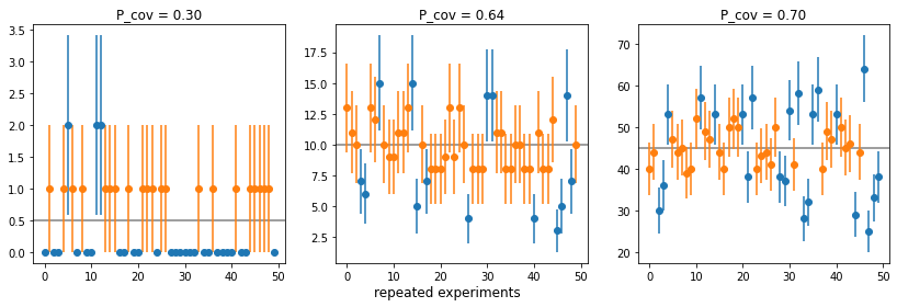
- Poisson interval \(N \pm \sqrt{N}\) only has proper coverage for \(N \gtrsim 45\)
- Reason: if \(N\) fluctuates downwards, interval shrinks
- Intervals can be empty in some experiments; this is not ideal, but not a defect
- If you have an estimate \(\mu\) for the true value of \(N_i\), this is better: \(N_i \pm \sqrt{\mu}\)
import numpy as np
import matplotlib.pyplot as plt
from scipy.stats import poisson

N = [0.5, 10, 20]
K = 100000

data = []
for Ni in N:
    n = poisson(Ni).rvs(size=K, random_state=int(Ni))
    mu = np.mean(n)
    sigma_est = np.sqrt(mu)
    inside = np.abs(Ni - n) < sigma_est
    cov_prob = np.mean(inside)
    data.append((Ni, n, sigma_est * np.ones(len(n)), inside, cov_prob))
plot()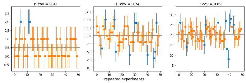
Maximum-likelihood estimator (MLE)
MLE has attractive properties
- For \(N \to \infty\), as close to true value as possible (proven)
- Unbiased and minimum variance
- In finite samples
- Biased in general, but bias zero or small for many important distributions
- Probably as close to true value as possible (conjecture)
- Easy to compute MLE and its variance estimate (with suitable software)
- But: Not robust against outliers or model misspecification
- For \(N \to \infty\), as close to true value as possible (proven)
Maximum-likelihood estimator for parameter \(a\) \[ \begin{aligned} h_\text{MLE}[x] &= \text{argmax}_{a}\, \ln \mathcal L(a) \\ \ln \mathcal L(a) &:= \ln \prod_i P(x_i; a) = \sum_i \ln f(x_i; a) + \text{const} \end{aligned} \]
MLE example: arithmetic mean is MLE for parameter \(\mu\) of normal distribution \[ \begin{aligned} \frac\partial{\partial \mu} \sum_i \ln\left( \frac1{\sqrt{2\pi} \sigma} \exp\left(-\frac{(x_i - \mu)^2}{2\sigma^2} \right)\right) &\overset{!}{=} 0 \\ \underbrace{\frac\partial{\partial \mu} \sum_i \ln\left( \frac1{\sqrt{2\pi} \sigma} \right)}_{0} - \frac\partial{\partial \mu} \sum_i \frac{(x_i - \mu)^2}{2\sigma^2} &= 0\\ \sum_i \frac{x_i - \mu}{\sigma^2} &= 0 \\ \sum_i x_i - \sum_i\mu &= 0 \\ \Rightarrow \hat\mu = \frac 1 N \sum_i x_i & \end{aligned} \]
In general: Use numerical optimiser (e.g. MINUIT) to find MLE for any distribution
Uncertainty of maximum likelihood estimate
- Two ways to compute uncertainty estimates for MLE based on theorems by Fisher and Wilks
- Recommended: lecture on MLE by Geyer (2013) https://www.stat.umn.edu/geyer/5601/notes/sand.pdf
Variance estimate
Variance estimate for MLE estimator \(\hat a\) of parameter \(a\) \[ \hat V[\hat a] = -\left(\frac{\partial^2 \ln \mathcal L(a)}{\partial a^2}\Bigg|_{a=\hat a}\right)^{-1} \]
Covariance estimate for multivariate MLE of parameter \(\vec a\) \[ \hat C_{ik}[\hat{\vec a}] = -\left(\frac{\partial^2 \ln \mathcal L(\vec a)}{\partial a_i \partial a_k}\Bigg|_{\vec a=\hat {\vec a}}\right)^{-1} \]
MINUIT computes this numerically (HESSE method)
Example: variance estimate for \(\hat\mu\) for normally distributed data with known width \(\sigma\) \[ -\left(\frac{\partial^2 \ln \mathcal L(\mu)}{\partial \mu^2}\right)^{-1} = \dots = \left(\frac{\partial^2}{\partial \mu^2} \sum_i \frac{(x_i - \mu)^2}{2\sigma^2}\right)^{-1} \] \[ = -\left(\frac{\partial}{\partial \mu} \sum_i \frac{(x_i - \mu)}{\sigma^2}\right)^{-1} = \left(\sum_i \frac1{\sigma^2}\right)^{-1} = \frac{\sigma^2}{N} \]
Well-known result for error on the mean
Profile likelihood scan
Produces asymmetric uncertainty intervals in general
For desired confidence level \(CL\) (a probability) solve \(\chi^2(\lambda;M) = CL\) for \(\lambda\), where \(M\) is number of parameters of interest (subset of all parameters)
Solve for contour in \(\vec a\)-space (parameters of interest) $$
2 = $$ where \(\hat b(\vec a)\) are maximum-likelihood estimates of nuisance parameters \(\vec b\) for fixed values of \(\vec a\)
Too complicated? No problem, MINUIT computes all this numerically for you (MINOS method)
Commonly used to draw uncertainty contours
Sometimes advertised as superior to variance estimate (HESSE method), but isn’t
- Does not produce intervals with better coverage in general
- Cannot combine asymmetric intervals/confidence regions from different experiments, see Roger’s lecture (references at the end)
If you really need this, publish full likelihood function with tools like pyhf or HistFactory
# Example: fit parameters of shifted Student's t distribution
import numpy as np
import matplotlib.pyplot as plt
from iminuit import Minuit
from iminuit.cost import UnbinnedNLL
from scipy.stats import t

nd = 3
mu = 1.0
sample = t(nd, mu).rvs(size=50, random_state=1)
def model(x, nd, mu):
return t(nd, mu).pdf(x)
cost = UnbinnedNLL(sample, model)
m = Minuit(cost, nd=2, mu=0)
m.limits["nd"] = (1, None)
m.migrad() # also runs equivalent of m.hesse() by default
m.minos()| Migrad | ||||
|---|---|---|---|---|
| FCN = 165 | Nfcn = 131 | |||
| EDM = 2.85e-05 (Goal: 0.0002) | ||||
| Valid Minimum | No Parameters at limit | |||
| Below EDM threshold (goal x 10) | Below call limit | |||
| Covariance | Hesse ok | Accurate | Pos. def. | Not forced |
| Name | Value | Hesse Error | Minos Error- | Minos Error+ | Limit- | Limit+ | Fixed | |
|---|---|---|---|---|---|---|---|---|
| 0 | nd | 3.6 | 1.5 | -1.2 | 2.1 | 1 | ||
| 1 | mu | 0.97 | 0.16 | -0.16 | 0.16 |
| nd | mu | |||
|---|---|---|---|---|
| Error | -1.2 | 2.1 | -0.16 | 0.16 |
| Valid | True | True | True | True |
| At Limit | False | False | False | False |
| Max FCN | False | False | False | False |
| New Min | False | False | False | False |
| nd | mu | |
|---|---|---|
| nd | 2.36 | 0.00743 (0.030) |
| mu | 0.00743 (0.030) | 0.0264 |
xm = np.linspace(-10, 10, 1000)
plt.hist(sample, bins=20, density=True, label="sample")
plt.plot(xm, t(*m.values).pdf(xm), label="fit")
plt.plot(xm, t(nd, mu).pdf(xm), label="truth")
plt.legend();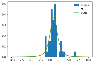
fig, ax = plt.subplots(1, 2, figsize=(14, 4))
for axi, par in zip(ax, ("nd", "mu")):
    plt.sca(axi)
    m.draw_mnprofile(par)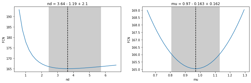
Misspecified models
Maximum-likelihood method assumes that model is correctly specified, all proven properties rely on that
Examples of misspecified models
- Assumed: signal only, actually: signal + background
- Assumed: normal distribution, actually: distorted normal (wider tails, asymmetric, etc)
If model is misspecified
- MLE is biased in general, but may not be
- MLE uncertainties (from either method) no longer have coverage
Fundamentalist: models are essentially always misspecified, since they are always approximations
Pragmatist: Small deviations have negligible effect
Worse at HL-LHC: higher statistics, so more sensitive to small deviations
- Need goodness-of-fit criterion (not discussed here) to check whether model is reliable
How to fix this: make model more general (by adding parameters) so it is no longer misspecified
- Use Student’s t (or double-sided Crystal Ball) instead of normal distribution to fit peak
- Use polynomial of higher order for smooth background
- …
Systematic uncertainties: Known unknowns
 * Donald Rumsfeld: “There are known knowns, things we know that we know; and there are known unknowns, things that we know we don’t know. But there are also unknown unknowns, things we do not know we don’t know.”
Why data analyses take so long: Study data, detector, and methods to turn unknown unknowns into known knowns or known unknowns
No formal way, but generally…
- Apply checks
- Split data by magnet polarity, fill, etc., analyse splits separately, check for agreement
- Worry
- What could go wrong?
- What are my assumptions?
- Example: You take an efficiency or correction factor from simulation, but simulation differs from real experiment; perform control measurement or use standard LHCb control measurements
- Methods
- If feasible, start from first principles or use methods that are known to be optimal/robust
- Examples
- Use Maximum-likelihood instead of least-squares fit
- Use bootstrap estimate of error
- Apply checks
Guidelines for handling systematic errors
Error propagation
- You have vector of values \(\vec a\) with covariance matrix \(C_a\) and a smooth function \(\vec b = f(\vec a)\), you want to know \(C_b\)
- \(\vec b\) can have different dimensionality from \(\vec a\)
Option 1: Standard error propagation
Based on first order Taylor expansion \[ C_b = J \, C_a \, J^T \] with Jacobi matrix \(J\) \[ J_{ik} = \frac{\partial f_i}{\partial a_k} \]
For derivation, see F. James book (references at end)
Can be used for statistical and systematic uncertainties!
Useful special cases
- Sum of scaled independent random values \(c = \alpha a + \beta b\) (\(\alpha, \beta\) are constant) \[ \sigma^2_c = \alpha^2 \sigma^2_a + \beta^2 \sigma^2_b \]
- Product of powers of independent random values \(c = a^\alpha \, b^\beta\) \[ \left(\frac{\sigma_c}{c}\right)^2 = \alpha^2 \left(\frac{\sigma_a}{a}\right)^2 + \beta^2 \left(\frac{\sigma_b}{b}\right)^2 \]
- Dominated by component with largest (relative) uncertainty
- Put your effort in estimating largest component and be more lax on small components
Example
Arithmetic mean \[ \hat \mu = \frac 1N\sum_i x_i \]
Variance of x (unbiased formula for unkown mean) \[ \hat V[x] = \frac 1{N-1} \sum_i (x_i - \hat\mu)^2 \]
Variance of the mean \[ \hat{V}[\hat \mu] = \frac1{N^2} \sum_i \hat{V}[x_i] = \frac 1 {N(N - 1)}\sum_i (x_i - \hat \mu)^2 \]
Error-prone to do by hand, use software to compute numerical derivative
Option 2: Monte-Carlo propagation
To apply, you need to know distribution of \(\vec a\)
Randomly sample \(K\) times
Compute sample \(\{\vec b_k \} = \{ f(\vec a_k) \}\)
Compute sample covariance of \(\{\vec b_k \}\)
import numpy as np
from jacobi import propagate  # uses Option 1
from scipy.stats import multivariate_normal

a0, sigma_a0 = 2, 0.2
a1, sigma_a1 = 3, 0.5

a = [a0, a1]
cov_a = np.zeros((2, 2))
cov_a[0, 0] = sigma_a0 ** 2
cov_a[1, 1] = sigma_a1 ** 2

# option 1
b, cov_b = propagate(np.mean, a, cov_a)
print(f"option 1: b = {b:.2f} +/- {np.sqrt(cov_b):.2f}")

# option 2
a_sample = multivariate_normal(a, cov_a).rvs(size=10000)
b_sample = np.mean(a_sample, axis=1) # sum over second axis
cov_b = np.cov(b_sample, ddof=1)
print(f"option 2: b = {b:.2f} +/- {np.sqrt(cov_b):.2f}")
option 1: b = 2.50 +/- 0.27
option 2: b = 2.50 +/- 0.27- Results identical here because function was linear; they differ in general
- Which is better? Hard to say, depends on particular case
- Option 2 is conceptually better, but you may need very large samples (>10000) to beat option 1 in accuracy
LHCb Statistics Guidelines
- Living document on GitLab to collect information about best practices
- Everyone can edit this and propose new items!
- LHCb StatML conveners are editors, liaisons check new content
- Index instead of a book
- Brief items with advice
- Links to literature
- In conversation, you can directly link to items, point to title and copy link (right-click menu)
Introductory statistics books
List of books on TWiki pages of Statistis and Machine Learning WG
Books I personally learned from
- Glen Cowan, “Statistical Data Analysis”, Oxford University Press, 1998
- F. James, “Statistical Methods in Experimental Physics”, 2nd edition, World Scientific, 2006
- B. Efron, R.J. Tibshirani, “An Introduction to the Bootstrap”, CRC Press, 1994
Roger Barlow
More Jupyter notebooks
Free books