from sympy import *

n = symbols("n", integer=True, positive=True)
v = symbols("v", real=True, positive=True)


def poisson(n, v):
    return v ** n * exp(-v) / factorial(n)

poisson(n, v)
\(\displaystyle \frac{v^{n} e^{- v}}{n!}\)
For GoF tests, we often use a test statistic that is asymptotically \(\chi^2\) distributed.
We compute the test statistic on binned data with \(k\) bins with Poisson-distributed counts \(n_i\) for which we have estimates of the expected counts \(\nu_i\), typically obtained from a fitted model with \(m\) free parameters. If the data is truely sampled from the model (the \(H_0\) hypothesis), the test statistic \(X\) is asymptotically distributed as \(\chi^2(k - m)\).
Small p-values \(P = \int_{X}^\infty \chi^2(X'; k - m) \, \text{d}X'\) can be used as evidence against the hypothesis \(H_0\).
Note: the asymptotic limit is assumed to be taken while keeping the binning constant. If the binning is adaptive to the sample size so that \(\nu_i\) remains constant, \(X\) will not approach the \(\chi^2(k - m)\) distribution.
There are candidates for an asymptotically \(\chi^2\)-distributed test statistic.
Pearson’s test statistic \[ X_P = \sum_i \frac{(n_i - \nu_i)^2}{\nu_i} \]
Pearson’s test statistic with \(\nu_i\) replaced by bin-wise estimate \(n_i\) \[ X_N = \sum_i \frac{(n_i - \nu_i)^2}{n_i} \]
Likelihood ratio to saturated model (see e.g. introduction of https://doi.org/10.1088/1748-0221/4/10/P10009) \[ X_{L} = 2\sum_i \Big( n_i \ln\frac{n_i}{\nu_i} - n_i + \nu_i \Big) \] The statistic is equal to \(-2\ln(L/L_\text{saturated})\), with \(L = \prod_i P_\text{poisson}(n_i; \nu_i)\) and \(L_\text{saturated} = \prod_i P_\text{poisson}(n_i; n_i)\), the likelihood for the saturated model with \(\nu_i = n_i\). The saturated model has the largest possible likelihood given the data.
Transform-based test statistic \[ X_T = \sum_i z_i^2 \quad\text{with}\quad z_i = q_\text{norm}\bigg(\sum_{k=0}^{n_i} P_\text{poisson}(k; v_i)\bigg) \] where \(q_\text{norm}\) is the quantile of the standard normal distribution. The double-transform converts a Poisson distributed count \(k\) into a variable \(z\) that has a standard normal distribution.
from sympy import *
n = symbols("n", integer=True, positive=True)
v = symbols("v", real=True, positive=True)
def poisson(n, v):
return v ** n * exp(-v) / factorial(n)
poisson(n, v)\(\displaystyle \frac{v^{n} e^{- v}}{n!}\)
X_L = simplify(- 2 * (log(poisson(n, v)) - log(poisson(n, n)))); X_L\(\displaystyle 2 n \log{\left(n \right)} - 2 n \log{\left(v \right)} - 2 n + 2 v\)
Given this choice, it is fair to ask which test statistic performs best. The test statistics may approach the \(\chi^2(k - m)\) distribution with different speeds.
We check this empirically with toy simulations. For each toy experiment, we use a fixed expected value \(\nu_i = \mu\) and draw \(k\) Poisson-distributed numbers \(n_i\) from \(\mu\), corresponding to \(k\) bins in the toy experiment. We then compute the test statistics \(X\) and its p-value, assuming it is \(\chi^2(k)\) distributed (\(m = 0\) here). This is repeated many times to get a histogram of p-values. The distribution is uniform if the test statistic \(X\) is indeed \(\chi^2(k)\) distributed. Deviations from uniformity indicate that the test statistic has not reached the asymptotic limit yet.
We then quantify the agreement of the p-value distribution with a flat distribution with the reduced \(\chi^2\) value.
import numpy as np
import numba as nb
from scipy.stats import chi2, poisson, norm
import matplotlib.pyplot as plt
from pyik.mplext import plot_hist
# numba currently does not support scipy, so we cannot access
# scipy.stats.norm.ppf and scipy.stats.poisson.cdf in a JIT'ed
# function. As a workaround, we wrap special functions from
# scipy to implement the needed functions here.
from numba.extending import get_cython_function_address
import ctypes
def get(name, narg):
addr = get_cython_function_address("scipy.special.cython_special", name)
functype = ctypes.CFUNCTYPE(ctypes.c_double, *([ctypes.c_double] * narg))
return functype(addr)
erfinv = get("erfinv", 1)
gammaincc = get("gammaincc", 2)
@nb.vectorize('float64(float64)')
def norm_ppf(p):
return np.sqrt(2) * erfinv(2 * p - 1)
@nb.vectorize('float64(intp, float64)')
def poisson_cdf(k, m):
return gammaincc(k + 1, m)
# check implementations
m = np.linspace(0.1, 3, 20)[:,np.newaxis]
k = np.arange(10)
got = poisson_cdf(k, m)
expected = poisson.cdf(k, m)
np.testing.assert_allclose(got, expected)
p = np.linspace(0, 1, 10)
got = norm_ppf(p)
expected = norm.ppf(p)
np.testing.assert_allclose(got, expected)@nb.njit
def xn(n, v):
r = 0.0
k = 0
for ni in n:
if ni > 0:
k += 1
r += (ni - v) ** 2 / ni
return r, k
@nb.njit
def xp(n, v):
return np.sum((n - v) ** 2 / v), len(n)
@nb.njit
def xl(n, v):
r = 0.0
for ni in n:
if ni > 0:
r += ni * np.log(ni / v) + v - ni
else:
r += v
return 2 * r, len(n)
@nb.njit
def xt(n, v):
p = poisson_cdf(n, v)
z = norm_ppf(p)
return np.sum(z ** 2), len(n)
@nb.njit(parallel=True)
def run(n, mu, nmc):
args = []
for i in range(len(n)):
for j in range(len(mu)):
for imc in range(nmc):
args.append((i, j, imc))
results = np.empty((4, len(n), len(mu), nmc, 2))
for m in nb.prange(len(args)):
i, j, imc = args[m]
ni = n[i]
mui = mu[j]
np.random.seed(imc)
x = np.random.poisson(mui, size=ni)
rp = xp(x, mui)
rn = xn(x, mui)
rl = xl(x, mui)
rt = xt(x, mui)
results[0, i, j, imc, 0] = rp[0]
results[0, i, j, imc, 1] = rp[1]
results[1, i, j, imc, 0] = rn[0]
results[1, i, j, imc, 1] = rn[1]
results[2, i, j, imc, 0] = rl[0]
results[2, i, j, imc, 1] = rl[1]
results[3, i, j, imc, 0] = rt[0]
results[3, i, j, imc, 1] = rt[1]
return results
mu = np.geomspace(1e-1, 1e3, 17)
n = 1, 3, 10, 30, 100, 1000
nmc = 10000
result = run(n, mu, nmc)def reduced_chi2(r):
p = 1 - chi2.cdf(*np.transpose(r))
bins = 20
xe = np.linspace(0, 1, bins + 1)
n = np.histogram(p, bins=xe)[0]
v = len(p) / bins
return np.sum((n - v) ** 2 / v) / bins
matrix = np.empty((len(result), len(n), len(mu)))
for k in range(len(result)):
for i, ni in enumerate(n):
for j, mui in enumerate(mu):
matrix[k, i, j] = reduced_chi2(result[k, i, j])def plot(r, **kwargs):
p = 1 - chi2.cdf(*np.transpose(r))
bins = 20
xe = np.linspace(0, 1, bins + 1)
n = np.histogram(p, bins=xe)[0]
plot_hist(xe, n, **kwargs)
for i, ni in enumerate(n):
for j, mui in enumerate(mu):
if j % 4 == 0: # draw only every forth value of mu
fig, ax = plt.subplots(1, 4, figsize=(15, 5))
plt.suptitle(f"k = {ni} mu = {mui:.2f}")
for k, t in enumerate("PNLT"):
plt.sca(ax[k])
plot(result[k, i, j])
plt.title(f"$X_{t}$ ($\chi^2/n_\mathrm{{dof}} = ${matrix[k, i, j]:.2g})")RuntimeWarning: More than 20 figures have been opened. Figures created through the pyplot interface (`matplotlib.pyplot.figure`) are retained until explicitly closed and may consume too much memory. (To control this warning, see the rcParam `figure.max_open_warning`).
fig, ax = plt.subplots(1, 4, figsize=(15, 5))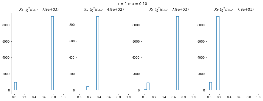
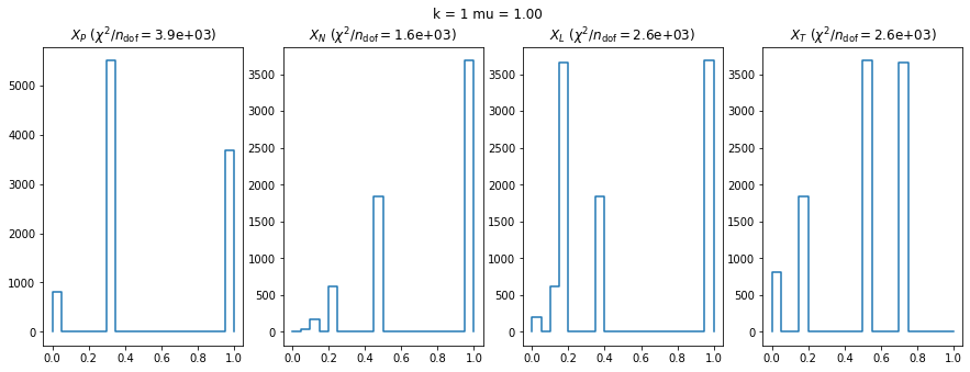
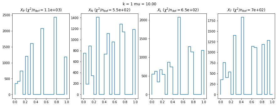
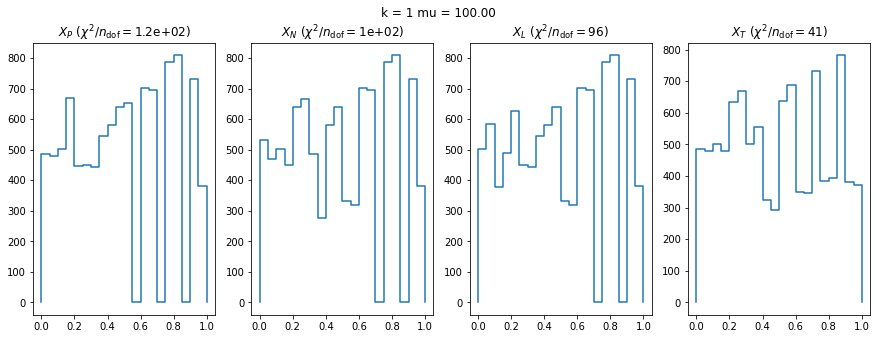
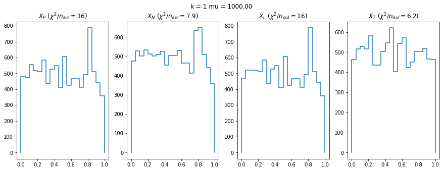
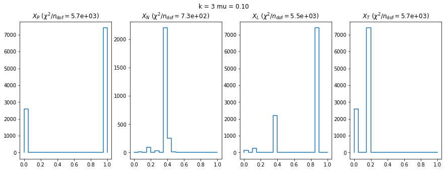
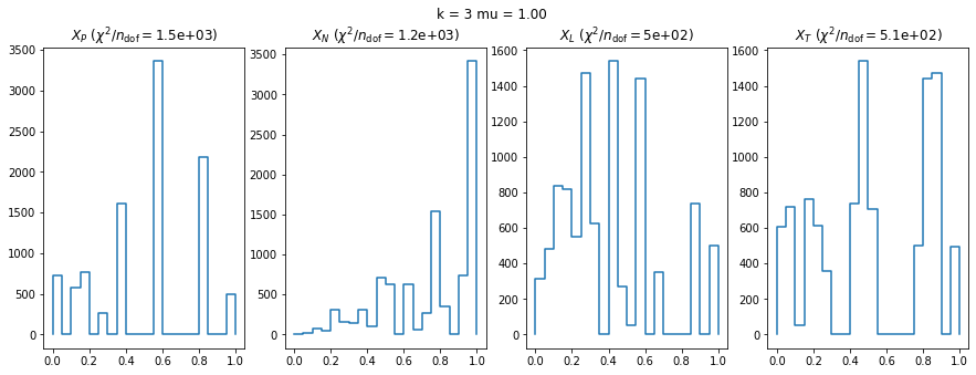
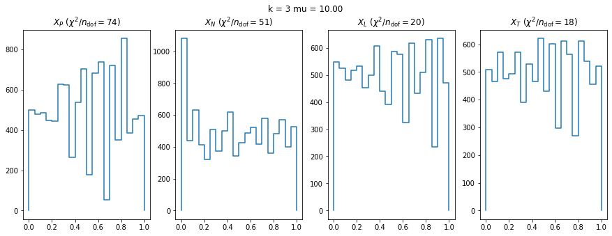
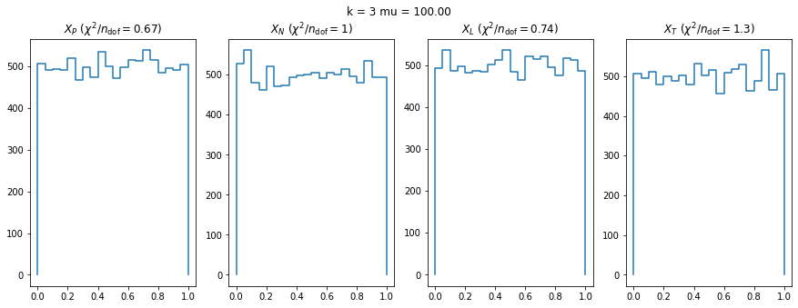
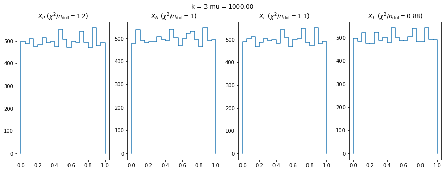
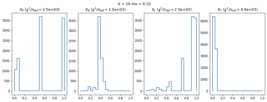
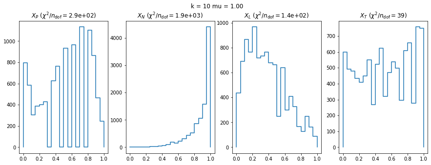
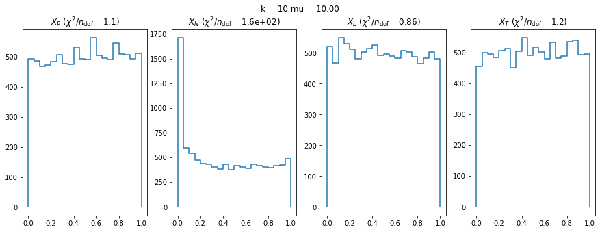
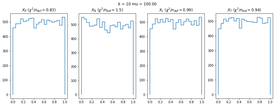
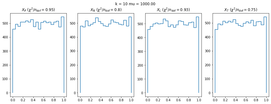
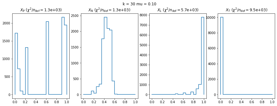
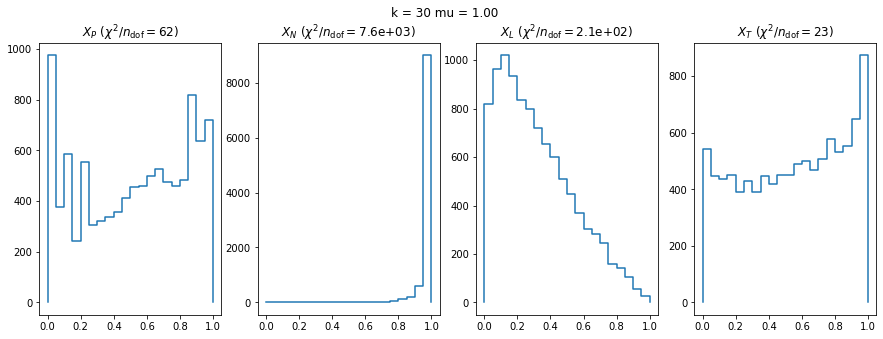
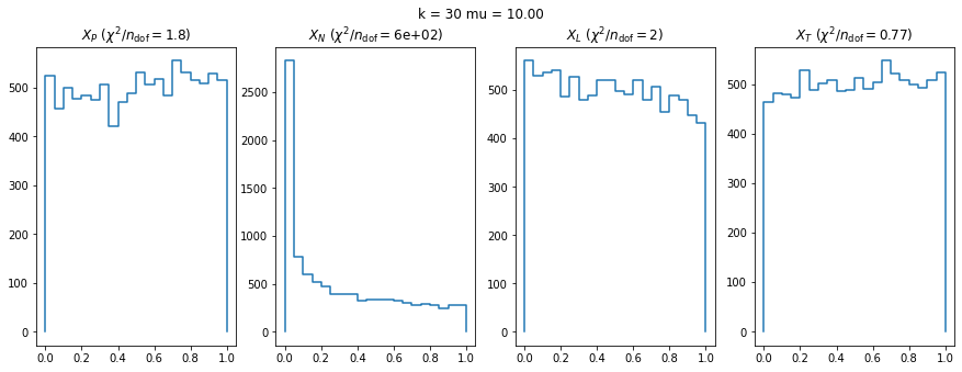
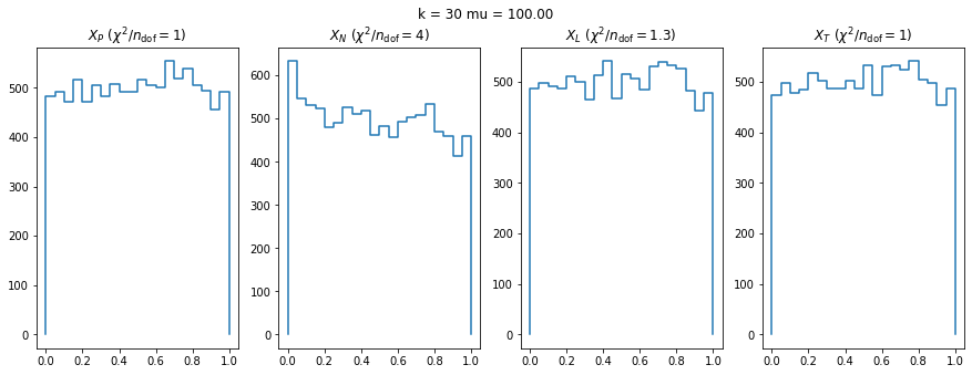
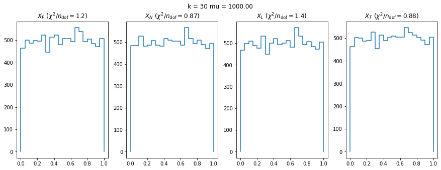
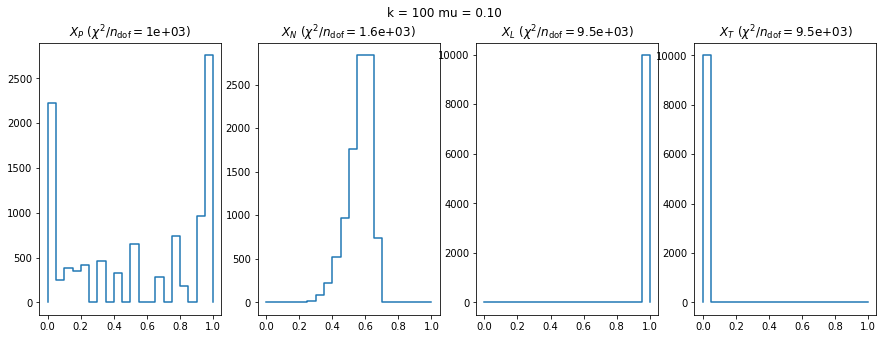
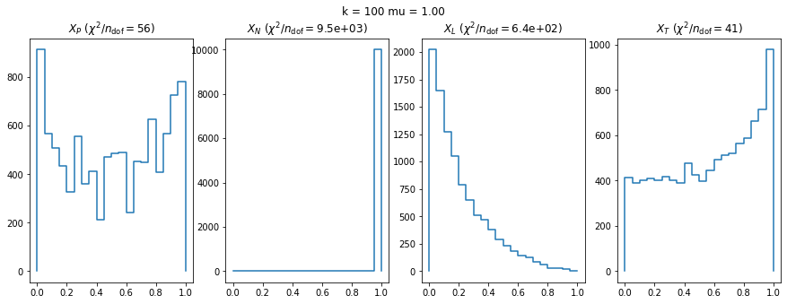
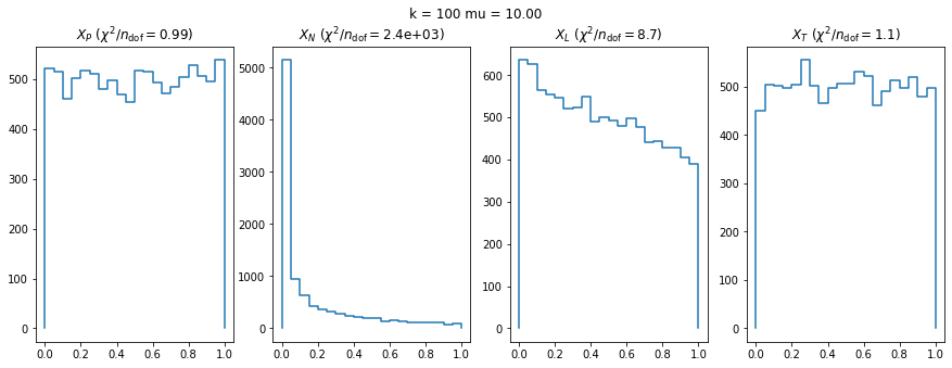
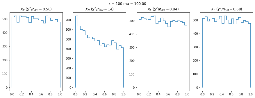
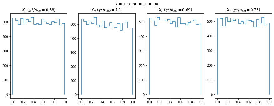
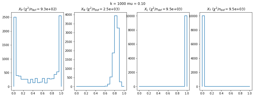
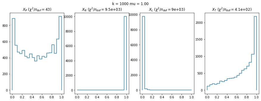
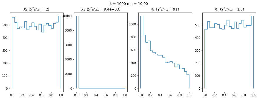
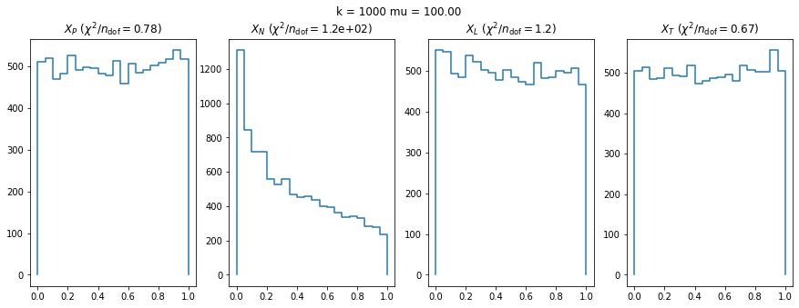
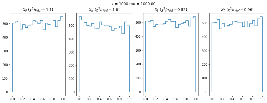
We can by eye that \(X_P\) gives the best results. Its p-value distribution converges to a uniform distribution for lower values of \(\mu\) and \(n\) than the other two test statistics. We summarize this by plotting the reduced \(\chi^2\) for flatness as a function of \(\mu\) and \(n\).
fig, ax = plt.subplots(1, len(result), figsize=(15, 5), sharex=True, sharey=True)
for i, ni in enumerate(n):
    for axi, matrixi in zip(ax, matrix):
        axi.plot(mu, matrixi[i],
                 label=f"$k = {ni:.1f}$")

for axi, t in zip(ax, "PNLT"):
    axi.set_title(f"$X_{t}$")
    axi.axhline(1, ls=":", color="0.5", zorder=0)
    axi.set_xlabel("$\mu$")
ax[0].set_ylabel("$\chi^2 / n_\mathrm{dof}$")
ax[1].legend()
plt.loglog();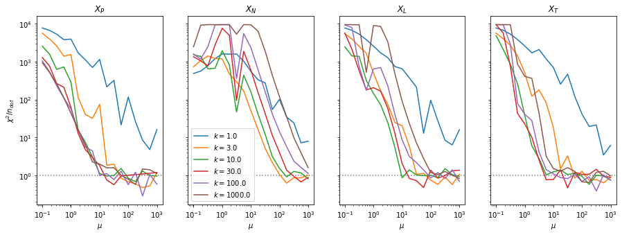
for i, ni in enumerate(n):
    plt.figure()
    plt.title(f"k = {ni}")
    for j, t in enumerate("PNLT"):
        plt.plot(mu, matrix[j, i] / matrix[0, i],
                 label=f"$X_{t}$")
    plt.loglog()
    plt.xlabel("$\mu$")
    plt.ylabel("red. $\chi^2$ ratio")
    plt.legend()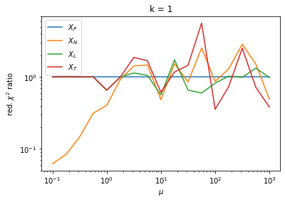
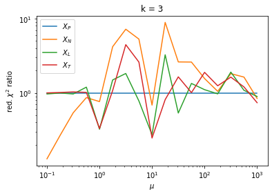
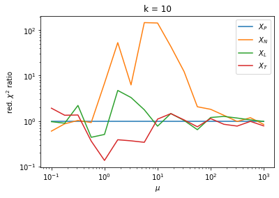
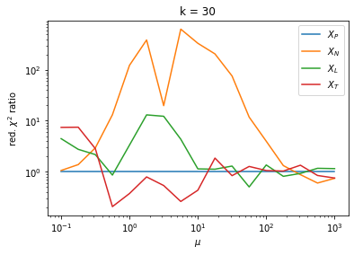
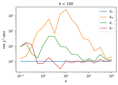
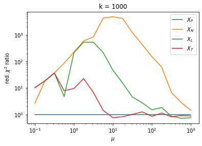
The classic test statistics \(X_P\) perform best overall, it converges to the asymptotic \(\chi^2\) distribution for smaller values of \(\mu\) and \(k\) and is also the simplest to compute.
The statistic \(X_L\) shows a curious behavior, it converges well around \(k=10\), on par with \(X_P\), but the convergence gets worse again for \(k > 10\).
The study confirms that none of the test statistics is doing well if the expected count per bin is smaller than about 10. If the original binned data contains bins with small counts, it is recommended to compute the distribution of the test statistic via parametric bootstrapping from the fitted model instead of using the asymptotic \(\chi^2\) distribution. Parametric bootstrapping in this case simplifies to drawing new samples for each data bin from a Poisson distribution whose expectation is equal to the expected count per bin predicted by the model. For many such samples one computes the test statistic to obtain a distribution. The p-value is then given by the fraction of sample values that are higher than the original value.