Solving the duffing oscillator

Here I solve the differential equations for the duffing oscillator with scipy and animate the solution with matplotlib. The oscillator exhibits chaotic behavior.

import numpy as np
from scipy.integrate import solve_ivp
import matplotlib.pyplot as plt
from matplotlib import animation

alpha = -1
beta = 1
gamma = 0.1
omega = 1.4
# interesting values for epsilon: 0.1, 0.4, 1.0
epsilon = 0.4


def V(x):
    return alpha * x ** 2 / 2 + beta * x ** 4 / 4

def ode(t, y):    
    x, xdot = y
    xdotdot = -(gamma * xdot + alpha * x + beta * x ** 3)
    xdotdot += epsilon * np.cos(omega * t)
    return xdot, xdotdot

# solve equation of motion

x0, v0 = 0, 0
n_samples_per_period = 50
n_period = 100
period = 2 * np.pi / omega
tmax = n_period * period

t = np.linspace(0, tmax, n_samples_per_period * n_period)
sol = solve_ivp(ode, (0, tmax), (x0, v0), t_eval=t)

x, xdot = sol.y

# setup animation
fig, ax = plt.subplots(2, 2)

plt.sca(ax[0,0])
plt.title("potential energy")
xext = max(np.max(np.abs(x)) * 1.05, 1.5)
x1 = np.linspace(-xext, xext)
y1 = V(x1)
plt.plot(x1, y1)
ln1, = plt.plot([], [], 'mo')
plt.xlabel(r'$x$')
plt.ylabel(r'$V(x)$')
plt.xlim(-xext - 0.05, xext + 0.05)
plt.ylim(np.min(y1) - 0.05, np.max(y1))

ax2 = ax[1, 0]
plt.sca(ax2)
plt.title("position vs. time")
plt.xlabel(r'$t$')
plt.ylabel(r'$x$')
ln2, = plt.plot([], [])
plt.ylim(-xext, xext)

plt.sca(ax[0, 1])
plt.title("Poincaré section")
plt.xlabel(r'$x$')
plt.ylabel(r'$\dot{x}$')
plt.scatter(x[::n_samples_per_period], xdot[::n_samples_per_period], s=1, lw=0)
plt.xlim(-xext, xext)
plt.ylim(np.min(xdot), np.max(xdot))

plt.sca(ax[1,1])
plt.title("phase space")
plt.xlabel(r'$x$')
plt.ylabel(r'$\dot{x}$')
ln3, = plt.plot([], [])
ln3a, = plt.plot([], [], 'mo')
plt.xlim(-xext, xext)
vext = np.max(np.abs(xdot))
plt.ylim(-vext, vext)

plt.tight_layout()

def animate(i):    
    ln1.set_data([x[i]], [V(x[i])])
    j = max(0, i - 10 * n_samples_per_period)
    sl = slice(j, i+1)
    ln2.set_data(t[sl], x[sl])
    ax2.set_xlim(t[j], t[i+1])
    sl = slice(0, i+1)
    ln3.set_data(x[sl], xdot[sl])
    ln3a.set_data([x[i]], [xdot[i]])
    return (ln1, ln2, ln3, ln3a)

anim = animation.FuncAnimation(fig, animate, frames=len(x), interval=2)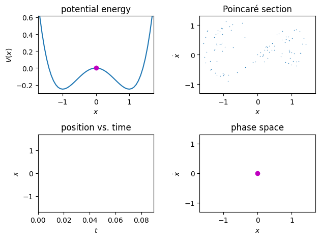

To see the animation in action, run this code in a Jupyter notebook and prepend the %matplotlib notebook to the first cell.