from iminuit import Minuit
from iminuit.cost import ExtendedUnbinnedNLL
from numba_stats import t, truncexpon, expon
import numpy as np
import numba as nb
import matplotlib.pyplot as pltThe logaddexp special function was made to perform this calculation more accurately: \[ y = \ln(\exp(a) + \exp(b)). \] This calculation occurs when we fit a mixed PDF with two components to a data sample, and both components can be modeled with PDFs from the exponential family. In that case, one can compute \(a\) and \(b\) efficiently, which represent the log-probability-density. This is not artificial, the normal, student’s t, and exponential distributions are from the exponential family.
Because of the finite dynamic range of floating point numbers and round-off, this computation can become inaccurate or yield infinity. One can avoid these issues by first determining whether \(a\) or \(b\) is larger and then by factoring it out of the equation. The logaddexp special function implements this strategy.
We explore this based on a toy example of a signal peak sampled from the student’s t distribution over an exponential background.
This is our toy data sample that we wish to fit.
rng = np.random.default_rng(1)

x = 0.1 * rng.standard_t(2, size=1000) + 1
x = np.append(x, rng.exponential(size=2000))
x = x[(0 < x) & (x < 2)]

plt.hist(x, bins=100);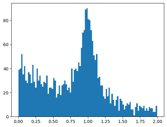
As a reference, we first run the standard fit without logaddexp.
def model(x, ns, df, mu, sigma, nb, tau):
    return ns + nb, ns * t.pdf(x, df, mu, sigma) + nb * truncexpon.pdf(
        x, 0, 2, 0, tau)


cost = ExtendedUnbinnedNLL(x, model)

m = Minuit(cost, ns=1000, nb=2000, df=2, mu=1, sigma=0.1, tau=1)
m.limits["ns", "nb", "sigma", "tau"] = (0, None)
m.limits["df"] = (1, None)
m.migrad()| Migrad | |
|---|---|
| FCN = -3.516e+04 | Nfcn = 170 |
| EDM = 8.76e-05 (Goal: 0.0002) | |
| Valid Minimum | Below EDM threshold (goal x 10) |
| No parameters at limit | Below call limit |
| Hesse ok | Covariance accurate |
| Name | Value | Hesse Error | Minos Error- | Minos Error+ | Limit- | Limit+ | Fixed | |
|---|---|---|---|---|---|---|---|---|
| 0 | ns | 930 | 50 | 0 | ||||
| 1 | df | 3.9 | 1.0 | 1 | ||||
| 2 | mu | 0.997 | 0.005 | |||||
| 3 | sigma | 0.103 | 0.006 | 0 | ||||
| 4 | nb | 1.80e3 | 0.06e3 | 0 | ||||
| 5 | tau | 1.04 | 0.05 | 0 |
| ns | df | mu | sigma | nb | tau | |
|---|---|---|---|---|---|---|
| ns | 2.35e+03 | -15.2 (-0.296) | -9.210e-3 (-0.036) | 111.09e-3 (0.354) | -1.4e3 (-0.517) | -0.8988 (-0.341) |
| df | -15.2 (-0.296) | 1.12 | 0.051e-3 (0.009) | 2.40e-3 (0.350) | 15.2 (0.253) | 0.0098 (0.170) |
| mu | -9.210e-3 (-0.036) | 0.051e-3 (0.009) | 2.78e-05 | -0.001e-3 (-0.024) | 9.206e-3 (0.031) | -0.023e-3 (-0.082) |
| sigma | 111.09e-3 (0.354) | 2.40e-3 (0.350) | -0.001e-3 (-0.024) | 4.2e-05 | -111.06e-3 (-0.302) | -0.07e-3 (-0.196) |
| nb | -1.4e3 (-0.517) | 15.2 (0.253) | 9.206e-3 (0.031) | -111.06e-3 (-0.302) | 3.22e+03 | 0.8986 (0.291) |
| tau | -0.8988 (-0.341) | 0.0098 (0.170) | -0.023e-3 (-0.082) | -0.07e-3 (-0.196) | 0.8986 (0.291) | 0.00296 |
Calling the logpdf methods for the two component PDFs is computationally more efficient than the pdf methods.
%%timeit
t.logpdf(x, 2, 0, 1)
27.8 µs ± 491 ns per loop (mean ± std. dev. of 7 runs, 10,000 loops each)%%timeit
t.pdf(x, 2, 0, 1)43.8 µs ± 3.19 µs per loop (mean ± std. dev. of 7 runs, 10,000 loops each)%%timeit
truncexpon.logpdf(x, 0, 2, 0, 1)8.12 µs ± 1.14 µs per loop (mean ± std. dev. of 7 runs, 100,000 loops each)%%timeit
truncexpon.pdf(x, 0, 2, 0, 1)21.4 µs ± 382 ns per loop (mean ± std. dev. of 7 runs, 10,000 loops each)Now we run the fit again using the logpdf methods of the component distributions and logaddexp. Our model now returns the log-probability and we notify the ExtendedUnbinnedNLL cost function of that fact with the keyword log=True.
def model_log(x, ns, df, mu, sigma, nb, tau):
    return ns + nb, np.logaddexp(
        np.log(ns) + t.logpdf(x, df, mu, sigma),
        np.log(nb) + truncexpon.logpdf(x, 0, 2, 0, tau))


cost_log = ExtendedUnbinnedNLL(x[(0 < x) & (x < 2)], model_log, log=True)

m_log = Minuit(cost_log, ns=1000, nb=2000, df=2, mu=1, sigma=0.1, tau=1)
m_log.limits["ns", "nb", "sigma", "tau"] = (0, None)
m_log.limits["df"] = (1, None)
m_log.migrad()| Migrad | |
|---|---|
| FCN = -3.516e+04 | Nfcn = 170 |
| EDM = 8.76e-05 (Goal: 0.0002) | |
| Valid Minimum | Below EDM threshold (goal x 10) |
| No parameters at limit | Below call limit |
| Hesse ok | Covariance accurate |
| Name | Value | Hesse Error | Minos Error- | Minos Error+ | Limit- | Limit+ | Fixed | |
|---|---|---|---|---|---|---|---|---|
| 0 | ns | 930 | 50 | 0 | ||||
| 1 | df | 3.9 | 1.0 | 1 | ||||
| 2 | mu | 0.997 | 0.005 | |||||
| 3 | sigma | 0.103 | 0.006 | 0 | ||||
| 4 | nb | 1.80e3 | 0.06e3 | 0 | ||||
| 5 | tau | 1.04 | 0.05 | 0 |
| ns | df | mu | sigma | nb | tau | |
|---|---|---|---|---|---|---|
| ns | 2.35e+03 | -15.2 (-0.296) | -9.210e-3 (-0.036) | 111.09e-3 (0.354) | -1.4e3 (-0.517) | -0.8988 (-0.341) |
| df | -15.2 (-0.296) | 1.12 | 0.051e-3 (0.009) | 2.40e-3 (0.350) | 15.2 (0.253) | 0.0098 (0.170) |
| mu | -9.210e-3 (-0.036) | 0.051e-3 (0.009) | 2.78e-05 | -0.001e-3 (-0.024) | 9.206e-3 (0.031) | -0.023e-3 (-0.082) |
| sigma | 111.09e-3 (0.354) | 2.40e-3 (0.350) | -0.001e-3 (-0.024) | 4.2e-05 | -111.06e-3 (-0.302) | -0.07e-3 (-0.196) |
| nb | -1.4e3 (-0.517) | 15.2 (0.253) | 9.206e-3 (0.031) | -111.06e-3 (-0.302) | 3.22e+03 | 0.8986 (0.291) |
| tau | -0.8988 (-0.341) | 0.0098 (0.170) | -0.023e-3 (-0.082) | -0.07e-3 (-0.196) | 0.8986 (0.291) | 0.00296 |
As expected, the results are identical up to round-off error. However, the computation should now be more numerically stable. Despite the fact that the logpdf is faster to compute, computing the log-likelihood is a bit slower. It is possible that the branch inside logaddexp slows down the computation.
%%timeit
cost(*m.values)
113 µs ± 13.5 µs per loop (mean ± std. dev. of 7 runs, 10,000 loops each)%%timeit
cost_log(*m_log.values)140 µs ± 1.5 µs per loop (mean ± std. dev. of 7 runs, 10,000 loops each)It is difficult to show that the second computation is more numerically stable. I make an attempt here by running the fit many times with variable starting values. This should lead to a valid more often if the computation is numerically stable. However, both versions of the fit perform equally well in this test.
rng = np.random.default_rng(1)
valids = np.empty((100, 2), dtype=bool)
for i in range(len(valids)):
    m.reset()
    m_log.reset()

    ns = rng.exponential(1000)
    df = 1 + rng.exponential(1)
    mu = rng.normal(1, 0.25)
    sigma = rng.exponential(0.1) + 0.01
    nb = rng.exponential(2000)
    tau = rng.exponential(1)

    m.values = (ns, df, mu, sigma, nb, tau)
    m.migrad()

    m_log.values = (ns, df, mu, sigma, nb, tau)
    m_log.migrad()

    valids[i, 0] = m.valid
    valids[i, 1] = m_log.valid
print(np.mean(valids, axis=0))
[0.99 0.99]The reason for this is that ExtendedUnbinnedNLL has some tricks (mostly the safe_log) which make sure that the simpler, less numerically stable, calculation also works most of the time.