from numba_stats import truncexpon, voigt
from scipy.stats import chi2, norm as scipy_norm
import numpy as np
from iminuit import Minuit
from iminuit.cost import ExtendedBinnedNLL
from matplotlib import pyplot as plt
from scipy.optimize import NonlinearConstraint
from jacobi import propagate
from resample.bootstrap import resample, variance
from skimage.measure import euler_number
from joblib import delayed, Parallel
from pathlib import Path
import pickle
import gzip
from rich.progress import ProgressWhen searching for an excess (peak) in some phase-space which has an unknown location, one has to correct the local significance for the fact that one would have reported random peaks produced by chance in the entire phase-space if these peaks were as large as the observed one. The result is called global significance. It is possible to compute the global significance with Monte-Carlo simulation, but this is expensive.
Gross and Vitells give a recipe for a surprisingly simple approximate calculation of global significance, which in its simplest form requires no Monte-Carlo simulation. One merely has to scan over the phase-space and count the number of upcrossings of the local significance of a small threshold. The accuracy of the method can be improved by running a small number of simulations.
This notebook applies the results from these two papers to a toy example
- E. Gross, O. Vitells, “Trial factors for the look elsewhere effect in high energy physics”, Eur. Phys. J. C 70 (2010) 525
- O. Vitells and E. Gross, “Estimating the significance of a signal in a multi-dimensional search”, Astropart. Phys. 35 (2011) 230, arXiv:1105.4355
and includes small refinements discussed in this presentation
- E. Gross, “Look Elsewhere Effect”, https://indico.cern.ch/event/353906/contributions/2219986/attachments/1329859/1997990/Thessaloniki_LEE_V1.pdf
The toy example is a search for a resonance in a wide mass window filled with background. Let’s assume that an experiment has found a peak in this window that does not correspond to a known particle. Of interest is the global significance of this peak. The model for the peak is a voigtian, which has two unknown parameters: the location of the peak, equal to the mass of the particle, and the width of the Cauchy distribution, related to the unknown life-time of the particle. The third parameter of the voigtian, the width of the Gaussian part, is assumed to be known, since it corresponds to the resolution of the experiment.
Prelude: technical obstacles and their solutions
Numerical issues when converting between large sigmas and small probabilities
In the calculation, the chi2 distribution is evaluated in its upper tail (and the standard normal, where the same issue occurs). Computing the p-value as 1 - chi2(...).cdf(z ** 2) becomes inaccurate when z is large. To fix this, one has to use the survival function implemented in scipy.stats, which calculates 1 - cdf accurately. Likewise, chi2(...).isf is used to compute the inverse of the survival function.
fig, ax = plt.subplots(1, 2, figsize=(12, 4))
plt.sca(ax[0])
z = np.linspace(0, 100)
plt.title("chi2(1)")
plt.plot(z, chi2(1).sf(z**2), label="sf")
plt.plot(z, 1 - chi2(1).cdf(z**2), label="1-cdf", ls="--")
plt.loglog()
plt.xlabel("z")
plt.ylabel("p-value")
plt.legend()

plt.sca(ax[1])
plt.title("chi2(1)")
p = np.geomspace(1, 1e-100)
plt.plot(p, chi2(1).isf(p) ** 0.5, label="isf(p)")
plt.plot(p, chi2(1).ppf(1 - p) ** 0.5, label="ppf(1-p)", ls="--")
plt.loglog()
plt.xlabel("p-value")
plt.ylabel("z")
plt.legend();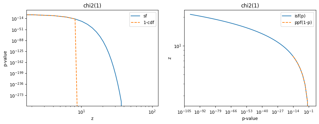
The same numerical issue also occurs when p-values are converted to sigmas using the integral of the upper tail of a standard normal distribution. The following two functions convert between p-values and z, the significance in units of standard deviation of a normal distribution. They will be used very often.
def z_to_pvalue(z):
    return scipy_norm.sf(z)


def pvalue_to_z(pvalue):
    return scipy_norm.isf(pvalue)
The quantity \(q = z^2\) is chi2 distributed with one degree of freedom. Only a positive excess is counted in this study as evidence against the background-only hypothesis, but the chi2 distribution ignores the sign of the deviation. One can nevertheless obtain the same mapping between probabilities and sigmas by taking half of the p-value for the chi2 distribution. This identity will be important later.
from scipy.stats import norm

z = 5
q = z ** 2

norm().sf(z), 0.5 * chi2(1).sf(q)
(2.8665157187919333e-07, 2.8665157187919375e-07)Locally negative densities
In the scan over the parameter space, one has to fit the model µ s + b, where µ is the signal amplitude, s is the signal shape, and b is the background density. To avoid issues with Wilks’ theorem, fit is allowed to find peaks with µ < 0, even though they are not considered as evidence against the background-only hypothesis. This, however, also opens the technical possibility that the sum of signal and background densities locally becomes negative during the numerical minimization process, which is forbidden, as densities cannot be negative. If this happens, the fit would likely fail.
To work around this, a standard minimization is performed first with iminuit using the MIGRAD algorithm, but if that fails, scipy minimizers are called that support additional constrains which prevent the density from becoming locally negative. iminuit wraps these to make that simple. Minimization with MIGRAD is preferred, however, because MIGRAD is faster than the scipy minimizer with constraints. Having a fast and stable fit is beneficial, since millions of fits are run in this notebook, and it is important that the fit converges every time.
Computing the test statistic \(q\)
The computation of global significance is based on the local test statistic \(q\), which must be chi2 distributed. This test statistic can be computed in two ways, but the first way presented now is more accurate and is generally recommended.
The test statistic \(q\) appears in the likelihood ratio test, in which the likelihood of the background only hypothesis, where the signal amplitude is zero, is compared to the likelihood of the alternative hypothesis where the amplitude is non-zero. According to Wilks’ theorem, the quantity \(q\) is asymptotically chi2 distributed with one degree of freedom, \[ q = -2 \ln\frac{\mathcal{L}(0, \theta, \hat \phi')}{\mathcal{L}(\hat \mu, \theta, \hat \phi)}\,, \] where \(\mathcal{L}(\mu, \theta, \phi)\) is the likelihood for both hypotheses, \(\hat \mu\) is the best-fit value of the signal amplitude, \(\theta\) are any number of nuisance parameters fixed in the scan, and \(\hat \phi\) and \(\hat \phi'\) are best fit values of the parameters of the background model for the two hypotheses. These can take different values depending on whether \(\mu\) is zero or not, hence they are distinguished as \(\hat \phi\) and \(\hat \phi'\).
Note that \(q\) asymptotically follows a chi2 distribution with one degree of freedom for any lengths of the parameter vectors \(\theta\) and \(\phi\), since Wilks’ theorem only counts the difference in the number of free parameters between both hypotheses. This difference is always 1.
The second asymptotically equivalent way to compute \(q\) is to divide the signal amplitude by the signal uncertainty estimated by the fit, and to square the result: \[ q = \left(\frac{\hat \mu}{\hat \sigma_\mu}\right)^2 \] Note that \(z = \hat \mu / \hat \sigma_\mu\) is also the local significance in units of sigmas. However, numerical studies showed that this way of calculating \(q\) is less accurate and leads to deviations from the expected chi2 distribution in simulated experiments. The reason is that in practice the signal uncertainty is computed numerically from the second derivative of the log-likelihood, and is sometimes underestimated, leading to \(q\) values that are too large.
Construction of the dataset
The toy distribution is constructed. It is a background-only sample from a truncated exponential distribution. This random sample is called “data”, it shall represent the actual measurement which is scanned over for a peak.
lambd_true = 2000
background_true = 10000

data = truncexpon.rvs(1000, 4000, 0, lambd_true, background_true, 1)
plt.hist(data, bins=100)
plt.semilogy();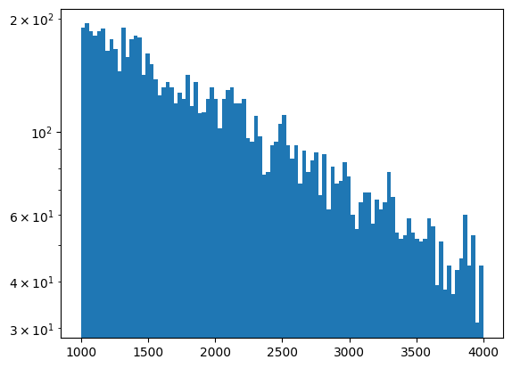
1D case
For the 1D case, I consider only the mass of the particle as unknown, but the width of the Cauchy distribution as known. I scan over the unknown mass and compute the local significance at each location. This requires fitting a signal + background model. I use iminuit and numba_stats, which works very well and is very fast, but other fitting frameworks can do the same job.
In case of iminuit, I use Minuit.fval to compute \(q\) which returns the value \(-2 \ln\mathcal{L}\) for the built-in cost function ExtendedBinnedNLL.
def model(xe, signal, mass, width, background, lambd):
    b = background * truncexpon.cdf(xe, 1000, 4000, 0, lambd)

    sigma_resolution = 50  # some fixed value

    # poor man's integration of voigt.pdf
    dx = np.diff(xe)
    ds = signal * voigt.pdf(xe[:-1] + 0.5 * dx, width, mass, sigma_resolution) * dx
    s = np.append(0, np.cumsum(ds))

    return s + b


def fit_background(mass):
    n, xe = np.histogram(mass, bins=100)
    c = ExtendedBinnedNLL(n, xe, model)
    minuit = Minuit(
        c, signal=0, mass=0, width=1, background=background_true, lambd=lambd_true
    )
    minuit.fixed["signal", "width", "mass"] = True
    minuit.limits["lambd", "background"] = (0, None)
    minuit.migrad()
    return minuit.fval, minuit


def fit(mass, m, w, chi2_background):
    n, xe = np.histogram(mass, bins=100)
    c = ExtendedBinnedNLL(n, xe, model)
    minuit = Minuit(
        c, signal=0, mass=m, width=w, background=background_true, lambd=lambd_true
    )
    minuit.fixed["width", "mass"] = True
    minuit.limits["lambd", "background"] = (0, None)
    minuit.migrad()
    # The pdf must not be negative. If MIGRAD fails, then usually because of that.
    # If that happens, I try again with with a constrained minimization,
    # see explaination above.
    if not minuit.valid:
        minuit.reset()
        minuit.scipy(
            constraints=[
                NonlinearConstraint(lambda *args: np.diff(model(xe, *args)), 0, np.inf)
            ]
        )
        if not minuit.valid:
            return np.nan, minuit

    # In theory, q is always positive, but it can take a tiny negative value in practice
    # due to numerical errors. I guard against that with the max function.
    q = max(chi2_background - minuit.fval, 0)

    # I want to return z instead of q, which is not necessary, but instructive. So I
    # take the square root here. The square-root of q is always positive, but I also
    # want to know the sign of the fitted amplitude for further analysis, so I copy it
    # over from the fitted signal.
    z = np.copysign(q ** 0.5, minuit.values["signal"])

    # This alternative calculation of z is more straight-forward but less accurate:
    # z = (minuit.values["signal"] / minuit.errors["signal"])
    return z, minuit


def z_scan(mass, m_grid, rw_grid):
    chi2_background = fit_background(mass)[0]
    X, Y = np.meshgrid(m_grid, rw_grid)
    fn = np.vectorize(lambda m, rw: fit(mass, m, m * rw, chi2_background)[0])
    Z = fn(X, Y).T
    return np.squeeze(Z)


m_grid = np.linspace(1200, 3800, 200)
# relative width of Cauchy part is fixed in 1D case, will be scanned over in 2D case
rw_grid = 0.05

z = z_scan(data, m_grid, rw_grid)
Let’s plot the most significant peak candidate.
imax = np.argmax(z**2)
zmax, minuit = fit(
    data, m_grid[imax], rw_grid * m_grid[imax], fit_background(data)[0]
)
minuit.visualize()
plt.title(f"z = {zmax:.2f}")
plt.xlabel("mass");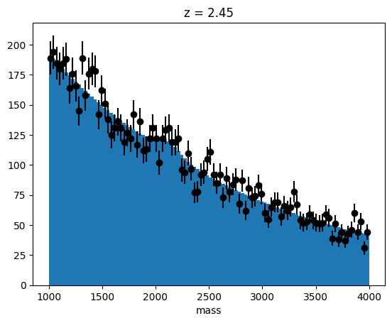
It has a local significance of \(z_\mathrm{local} = 2.45\).
Next, I plot the \(z\) values and the p-values computed from \(q = z^2\) and a chi2 distribution with one degree of freedom. From this I need to derive an excursion set, how many connected stretches (“upcrossings”) there are for which these p-values fall below threshold values computed from the one-sided standard normal distribution (these thresholds are given by the function z_to_pvalue). I emphasize that the p-value is computed from \(q\) using the chi2(1) distribution, but for the thresholds I use z_to_pvalue which gives half of chi2(1).sf(z ** 2).
This accounts for the fact that only positive \(z\) provide evidence against the background-only hypothesis. It also allows one to count the upcrossings at the lowest possible level of \(0\sigma\), which is mapped to the threshold P=0.5. These upcrossings occur very frequently and thus have a small relative counting error. This nice trick is not documented in the papers, but described in a presentation by Eilam Gross given at the ATLAS Stat Forum, 3/2010.
# p-value from chi2(1) for an excess in q=z^2
pvalue_q = chi2(1).sf(z ** 2)

fig, ax = plt.subplots(1, 2, figsize=(12, 4))
plt.sca(ax[0])
plt.axhline(0, ls="--", color="0.5")
plt.xlabel("mass / MeV")
plt.ylabel(r"$z_\mathrm{local}$")
plt.plot(m_grid, z)
plt.sca(ax[1])
plt.plot(m_grid, pvalue_q)
plt.semilogy()
plt.ylim(None, 1)
for sigma in range(5):
    # for thresholds, I use z_to_pvalue, see text
    p = z_to_pvalue(sigma)
    if p > np.min(pvalue_q):
        plt.axhline(p, ls="--", color="k")
        plt.text(
            3900, p, f"${sigma}\sigma$", fontsize="x-large", va="bottom", ha="right"
        )
plt.ylabel("p-value from chi2(1)")
plt.xlabel("mass / MeV")

z_local = z[imax]
print(f"z_local = {z_local:.2f} P_local = {z_to_pvalue(z_local):.3f}")
z_local = 2.45 P_local = 0.007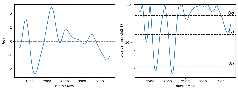
The following functions compute the number of upcrossings, the global significance, and the global p-value from the local significance values.
def compute_p_global(z, z_threshold, n_upcrossings):
    u = z**2
    u_threshold = z_threshold**2
    phalf = 0.5 * chi2(1).sf(u)  # equal to p_local = z_to_pvalue(z_local)
    return phalf + n_upcrossings * np.exp(0.5 * (u_threshold - u))


def compute_z_global(z, z_threshold, n_upcrossings):
    return pvalue_to_z(compute_p_global(z, z_threshold, n_upcrossings))


def compute_number_of_upcrossings(z, z_threshold):
    # I use euler_number from scikit-image to compute the number of upcrossings.
    # It is designed for 2D data, but also works on 1D data.
    excursion_set = chi2(1).sf(z ** 2) < z_to_pvalue(z_threshold)
    excursion_set = np.atleast_2d(excursion_set)
    return euler_number(excursion_set)


z_threshold = 0  # chosen threshold for upcrossings in units of sigma
n_upcrossings = compute_number_of_upcrossings(z, z_threshold)
print(f"upcrossings = {n_upcrossings}")

# propagate uncertainty of n_upcrossing, which is a Poisson distributed number
z_global, z_global_cov = propagate(
    lambda n: compute_z_global(z_local, z_threshold, n), n_upcrossings, n_upcrossings
)

print(f"z_global = {z_global:.2f} ± {z_global_cov ** 0.5:.2f}")
upcrossings = 5
z_global = 0.66 ± 0.35The uncertainty of the computed global significance is statistical: the expected number of upcrossings was replaced with an estimate based on the observed number of upcrossings in only one sample.
This error can be reduced to any desired value by running more simulations and computing the average of the number of upcrossings from these simulations. With 100 simulations, the error can be reduced by a factor of 10 to 0.02, which is already almost negligible. If a larger local significance is extrapolated, the error of the global significance measured in units of sigma becomes smaller.
I now confirm the calculation with a toy simulation, in which I repeatedly simulate independent experiments, do the local scan, and record the largest \(q\) value found. This produces a sample of \(q\) values.
# I cache this calculation, since it takes a while
cache_file = Path("q_samples.pkl.gz")

if cache_file.exists():
    with gzip.open(cache_file) as f:
        q = pickle.load(f)
else:
    q = []

    seeds = 10000

    @delayed
    def run(iseed):
        mass = truncexpon.rvs(1000, 4000, 0, lambd_true, background_true, iseed)
        z = z_scan(mass, m_grid, rw_grid)
        return np.max(z**2)

    with Progress() as progress:
        q = Parallel(n_jobs=8)(run(iseed) for iseed in progress.track(range(seeds)))
    q = np.array(q)

    with gzip.open(cache_file, "w") as f:
        pickle.dump(q, f)

# check that all fits converged properly
np.mean(np.isnan(q))0.0Here is the distribution of the test statistic \(q\) over many independent experiments. For large \(q\) values it becomes an exponential distribution, as predicted by the Gross & Vitells formula.
plt.hist(q, bins=100)
plt.semilogy()
plt.xlabel("q");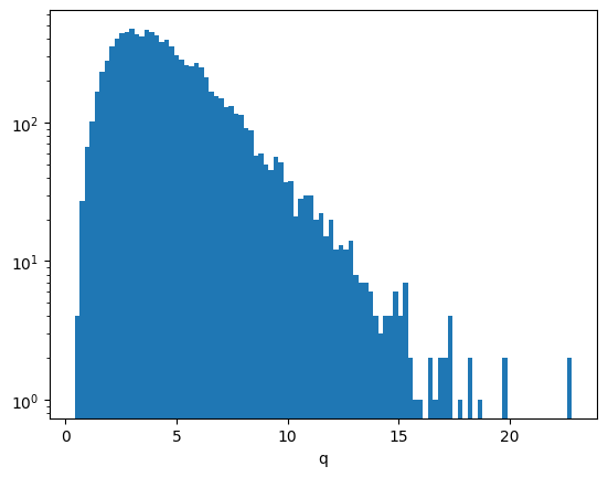
The global p-value is given by the fraction of \(q\) values in simulated experiments which exceed the value found in the original data sample. This probability is converted into sigmas with the usual conversion formula. The uncertainty is readily obtained with the bootstrap.
The simulation result is in agreement with the Gross & Vitells calculation.
p_global_sim = np.mean(q > z_local**2)
z_global_sim = pvalue_to_z(p_global_sim)

z_global_sim_cov = variance(lambda q: pvalue_to_z(np.mean(q > z_local**2)), q)
print(f"z_global_sim = {z_global_sim:.2f} +/- {z_global_sim_cov ** 0.5:.2f}")
z_global_sim = 0.73 +/- 0.01Out of curiosity, let’s plot the experiment with the largest \(q\). It turns out to be a negative deviation.
iseed = np.argmax(q)
mass = truncexpon.rvs(1000, 4000, 0, lambd_true, background_true, iseed)
z_m = []
for m in m_grid:
    z_m.append(fit(mass, m, rw_grid, fit_background(mass)[0]))
plt.plot(m_grid, [x[0] for x in z_m])
plt.ylabel("$z_\mathrm{local}$")
plt.xlabel("mass / MeV");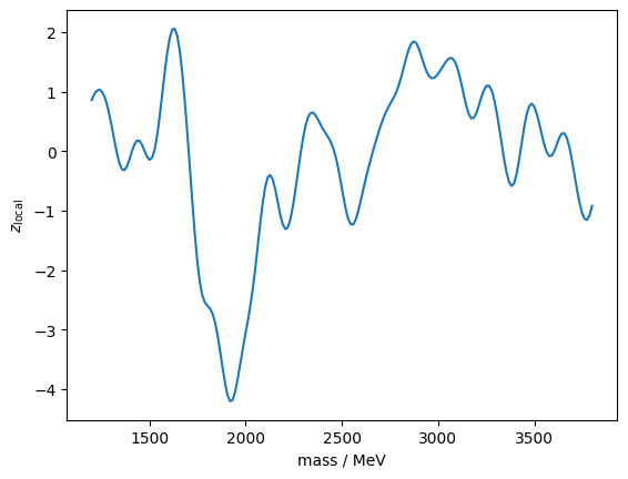
This is the corresponding fit of the maximum deviation:
z_m[np.argmax([x[0] ** 2 for x in z_m])][1]| Migrad | |
|---|---|
| FCN = 93.4 (χ²/ndof = 1.0) | Nfcn = 51 |
| EDM = 1.26e-05 (Goal: 0.0002) | |
| Valid Minimum | Below EDM threshold (goal x 10) |
| No parameters at limit | Below call limit |
| Hesse ok | Covariance accurate |
| Name | Value | Hesse Error | Minos Error- | Minos Error+ | Limit- | Limit+ | Fixed | |
|---|---|---|---|---|---|---|---|---|
| 0 | signal | -114 | 26 | |||||
| 1 | mass | 1.919e3 | 0.019e3 | yes | ||||
| 2 | width | 50.0e-3 | 0.5e-3 | yes | ||||
| 3 | background | 10.12e3 | 0.10e3 | 0 | ||||
| 4 | lambd | 1.97e3 | 0.05e3 | 0 |
| signal | mass | width | background | lambd | |
|---|---|---|---|---|---|
| signal | 655 | 0 | 0 | -0.8e3 (-0.288) | 0.1e3 (0.078) |
| mass | 0 | 0 | 0 | 0 | 0 |
| width | 0 | 0 | 0 | 0 | 0 |
| background | -0.8e3 (-0.288) | 0 | 0 | 1.09e+04 | -0.1e3 (-0.019) |
| lambd | 0.1e3 (0.078) | 0 | 0 | -0.1e3 (-0.019) | 2.22e+03 |
To verify the result of the Gross & Vitells formula more broadly, I compare the global p-values from the simulation and the computed ones from the formula for various values of \(q\). I use the bootstrap method to estimate the uncertainty of the simulation result, and numerical error propagation to compute the uncertainty of the Gross & Vitells formula.
Both results are in very good agreement above \(q > 7\), corresponding to \(z \approx 2.6\). The beauty of the Gross & Vitells formula is that it performs the best if \(z_\mathrm{local}\) is large, which is exactly the case where the classic simulation strategy becomes infeasible. The error on the Gross & Vitells formula can be easily reduced by a factor of 10, if the number of excursions is computed from an average of 100 background-only simulations (I don’t do that here).
q_grid = np.linspace(0, 25, 1000)

p = [np.mean(q > qi) for qi in q_grid]
plt.plot(q_grid, p, label="simulation")

p_err = variance(lambda q: [np.mean(q > qi) for qi in q_grid], q) ** 0.5
plt.fill_between(q_grid, p - p_err, p + p_err, fc="C0", alpha=0.5)

p2, p2cov = propagate(
    lambda n: compute_p_global(q_grid**0.5, z_threshold, n),
    n_upcrossings, n_upcrossings, diagonal=True
)
p2err = p2cov ** 0.5
plt.plot(q_grid, p2, label="Gross & Vitells")
plt.fill_between(q_grid, p2 - p2err, p2 + p2err, fc="C1", alpha=0.5)
plt.semilogy()
plt.ylabel("global p-value")
plt.xlabel("q = $z_\\mathrm{local}^2$")
plt.legend();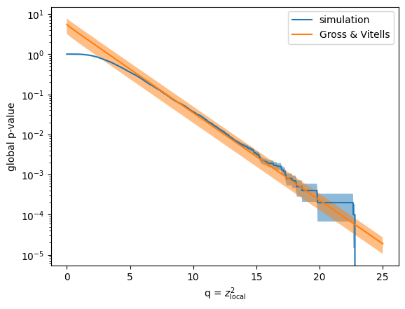
2D case
In HEP, one often has to scan over more than just the mass, the natural width of the peak is also unknown unless the life-time of the particle can be measured as well.
In this toy example, I scan over the relative width from 0 % to 10 % of the mass of the particle. One could equally well implement a scan where the width is independent of the mass.
I already wrote the scan function for the 1D case so that it also works for the 2D case. It is reused unmodified here.
m_grid = np.linspace(1200, 3800, 100)
rw_grid = np.linspace(0, 0.1, 20)

z = z_scan(data, m_grid, rw_grid)
z_local = np.max(z)
print(f"z_local = {z_local:.2f}")
z_local = 3.14A local excess of \(3.1\sigma\) is found, higher than the previous local excess found when the relative width was fixed. This is expected, it is more likely to find a large local deviation if the scanned parameter space is larger.
I visualize the result of the scan.
from matplotlib.colors import BoundaryNorm

cmap = plt.colormaps["bwr"]
norm = BoundaryNorm(np.linspace(-5, 5, 11), ncolors=cmap.N, clip=True)
plt.pcolormesh(m_grid, rw_grid, z.T, norm=norm, cmap=cmap)
plt.colorbar().set_label("z")
plt.title(f"z_local = {z_local:.2f}")
plt.xlabel("mass")
plt.ylabel("relative width");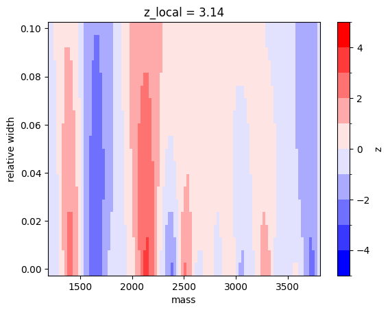
To apply the Gross & Vitells formula for the 2D case, excursion sets need to be computed again. An excursion set is obtained as before: the p-value is computed from \(q = z^2\) using the upper tail of the chi2(1) distribution, but the threshold probabilities are computed using the upper tail of a standard normal.
However, in a 2D plane, the excursions are counted differently. They are given by the number of locally connected excursions minus the number of holes. This difference is called the Euler characteristic.
Gross & Vitells describe a general algorithm to compute the Euler characteristic for any number of dimensions, which would take time to implement and test. Fortunately, I found an algorithm for the 2D case in the scikit-image Python library, which is a great time-saver.
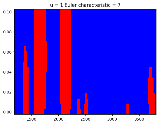
Shown below are the excursion sets for \(0\sigma\) and \(1\sigma\) and the computed Euler characteristic for these two binary images.
z_threshold = [0, 1]
euler_characteristic = []
for zt in z_threshold:
    excursions = chi2(1).sf(z**2) < z_to_pvalue(zt)
    ec = euler_number(excursions)  # euler_number is a misnomer by scikit-image
    euler_characteristic.append(ec)

    plt.figure()
    plt.pcolormesh(m_grid, rw_grid, excursions.T, cmap=cmap)
    plt.title(f"u = {zt} Euler characteristic = {ec}")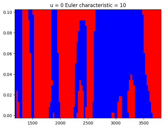
With these numbers I can again compute the extrapolation from local to global significance. I need to first solve a system of equations, for which one row is given by \[ N[\phi_u] = 1/2 P(\chi^2 > u) + (\mathcal{N}_1 + \mathcal{N}_2 \sqrt{u}) e^{-u/2}, \] where \(N[\phi_u]\) is the expected Euler characteristic for excursions above \(u = z_\mathrm{threshold}^2\), \(P(\chi^2 > u)\) is the upper tail integral of a chi2(1) distribution, and \(\mathcal{N}_1\), \(\mathcal{N}_2\) are unknown parameters for which I solve the system, using the estimated values \(N[\phi_u]\) for two chosen thresholds \(u_0 = 0\) and \(u_1 = 1\).
The system is linear in \(\mathcal{N}_1\) and \(\mathcal{N}_2\) and the solution readily obtained with standard algorithms. Once \(\mathcal{N}_1\) and \(\mathcal{N}_2\) are given, I can use the same formula to compute the global p-value (equal to \(N[\phi_u]\) for large \(u\)) from the local p-value (equal to \(1/2 P(\chi^2 > u)\)).
def compute_p_global(z_local, z_threshold, euler_characteristic):
    z_threshold = np.array(z_threshold)
    euler_characteristic = np.array(euler_characteristic)
    u = z_threshold ** 2
    p_chi2 = chi2(1).sf(u)

    # Solve system of linear equations
    # N[𝜙ᵤ] = 1/2 P(𝜒² > u) + (𝒩₁ + 𝒩₂ √𝑢) exp(−𝑢/2)
    # to get parameters 𝒩₁ and 𝒩₂.
    b = euler_characteristic - 0.5 * p_chi2
    f = np.exp(-u / 2)
    A = np.transpose((f, f * np.sqrt(u)))
    n1, n2 = np.linalg.solve(A, b)

    # I now apply
    # N[𝜙ᵤ] = 1/2 P(𝜒² > u) + (𝒩₁ + 𝒩₂ √𝑢) exp(−𝑢/2)
    # to the observed value of u = z_local^2.
    u = z_local**2
    f = np.exp(-u / 2)
    p_chi2 = chi2(1).sf(u)
    return 0.5 * p_chi2 + (n1 + n2 * np.sqrt(u)) * f


def compute_z_global(z_local, z_threshold, euler_characteristic):
    p_global = compute_p_global(z_local, z_threshold, euler_characteristic)
    return pvalue_to_z(p_global)


# Error propagation assumes that both Euler characteristics are 100% correlated.
# This is an approximation, but they must be strongly positively correlated.
z_global, z_global_cov = propagate(lambda n : compute_z_global(z_local, z_threshold, n),
                                   euler_characteristic,
                                   [euler_characteristic, euler_characteristic])

print(f"z_local = {z_local:.2f}")
print(f"z_global = {z_global:.2f} +/- {z_global_cov ** 0.5:.2f}")
z_local = 3.14
z_global = 1.23 +/- 0.26I check this result again using simulations of independent experiments as in the previous case. The simulation takes a long time now since each iteration is a scan over a 2D plane.
# I cache this calculation, since it takes a while
cache_file = Path("q_samples_2d.pkl.gz")

if cache_file.exists():
    with gzip.open(cache_file) as f:
        q = pickle.load(f)
else:
    q = []

    seeds = 10000

    @delayed
    def run(iseed):
        mass = truncexpon.rvs(1000, 4000, 0, lambd_true, background_true, iseed)
        z = z_scan(mass, m_grid, rw_grid)
        return np.max(z**2)

    with Progress() as progress:
        q = Parallel(n_jobs=8)(run(iseed) for iseed in progress.track(range(seeds)))
    q = np.array(q)

    with gzip.open(cache_file, "w") as f:
        pickle.dump(q, f)

# check that all fits converged properly
np.mean(np.isnan(q))0.0As expected, the distribution of \(q\) values approaches an exponential distribution for large \(q\).
plt.hist(q, bins=100)
plt.semilogy()
plt.xlabel("q");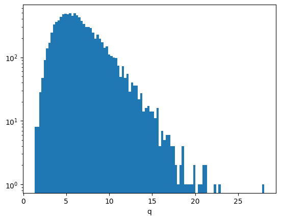
The simulation result is once again in excellent agreement.
p_global_sim = np.mean(q > z_local**2)
z_global_sim = pvalue_to_z(p_global_sim)

z_global_sim_cov = variance(lambda q: pvalue_to_z(np.mean(q > z_local**2)), q)
print(f"z_global_sim = {z_global_sim:.2f} +/- {z_global_sim_cov ** 0.5:.2f}")
z_global_sim = 1.25 +/- 0.02I plot again the scan with the most extreme local significance. It is a positive excess this time.
iseed = np.argmax(q)
mass = truncexpon.rvs(1000, 4000, 0, lambd_true, background_true, iseed)
z_m = []
for m in m_grid:
    z_m.append(fit(mass, m, rw_grid[0], fit_background(mass)[0]))
plt.plot(m_grid, [x[0] for x in z_m])
plt.ylabel("$z_\mathrm{local}$")
plt.xlabel("mass / MeV");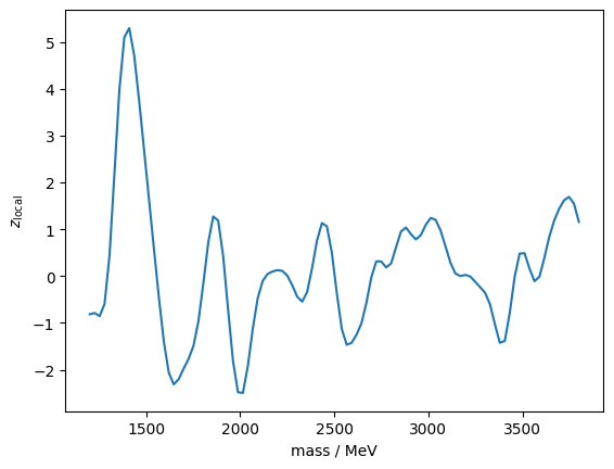
z_m[np.argmax([x[0] ** 2 for x in z_m])][1]| Migrad | |
|---|---|
| FCN = 95.07 (χ²/ndof = 1.0) | Nfcn = 52 |
| EDM = 3.11e-05 (Goal: 0.0002) | |
| Valid Minimum | Below EDM threshold (goal x 10) |
| No parameters at limit | Below call limit |
| Hesse ok | Covariance accurate |
| Name | Value | Hesse Error | Minos Error- | Minos Error+ | Limit- | Limit+ | Fixed | |
|---|---|---|---|---|---|---|---|---|
| 0 | signal | 180 | 40 | |||||
| 1 | mass | 1.410e3 | 0.014e3 | yes | ||||
| 2 | width | 0.0 | 0.1 | yes | ||||
| 3 | background | 9.82e3 | 0.10e3 | 0 | ||||
| 4 | lambd | 2.05e3 | 0.05e3 | 0 |
| signal | mass | width | background | lambd | |
|---|---|---|---|---|---|
| signal | 1.31e+03 | 0 | 0 | -1.1e3 (-0.298) | 0.5e3 (0.270) |
| mass | 0 | 0 | 0 | 0 | 0 |
| width | 0 | 0 | 0 | 0 | 0 |
| background | -1.1e3 (-0.298) | 0 | 0 | 1.1e+04 | -0.5e3 (-0.093) |
| lambd | 0.5e3 (0.270) | 0 | 0 | -0.5e3 (-0.093) | 2.9e+03 |
This indeed looks very much like a local resonance, but it is a random coincidence.
As before, I compute the global p-value using simulation and with the Gross & Vitells formula for various q-values to get a better picture of their agreement. The agreement is again very good above \(q > 7\), which corresponds to about \(2.6\sigma\).
q_grid = np.linspace(0, 25, 1000)

p = [np.mean(q > qi) for qi in q_grid]
plt.plot(q_grid, p, label="simulation")

p_err = variance(lambda q: [np.mean(q > qi) for qi in q_grid], q) ** 0.5
plt.fill_between(q_grid, p - p_err, p + p_err, fc="C0", alpha=0.5)

# We assume 100% correlation for both values of the Euler characteristic.
p2, p2cov = propagate(
    lambda n: compute_p_global(q_grid**0.5, z_threshold, n),
    euler_characteristic,
    [euler_characteristic, euler_characteristic],
)
p2err = np.diag(p2cov) ** 0.5
plt.plot(q_grid, p2, label="Gross & Vitells")
plt.fill_between(q_grid, p2 - p2err, p2 + p2err, fc="C1", alpha=0.5)
plt.semilogy()
plt.ylabel("global p-value")
plt.xlabel("q = $z_\\mathrm{local}^2$")
plt.legend();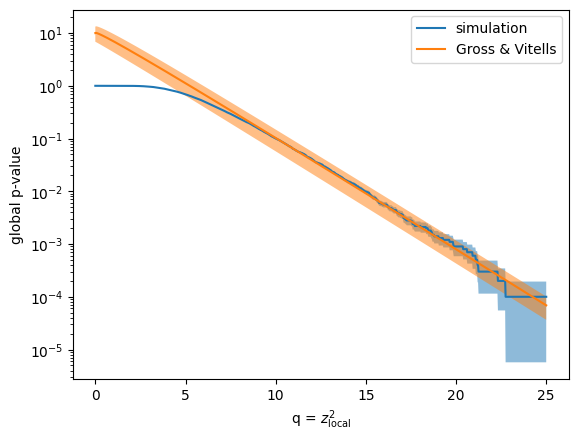
Conclusion
I explored the application of the Gross & Vitells formulas for signal models with one or two nuisance parameters (apart from the amplitude), which extrapolate a local significance for a signal found in 1D or 2D scans to a global significance.
Using iminuit and numba-stats, I implemented a fast and robust fit for a toy example, which consists of a model that mixes exponential background with a voigtian signal. The fits run fast and converge successfully every time, even though the total amount of fits run in this notebook is in the millions.
The Gross & Vitells formulas do not need my verification (they hold generally), but I needed to verified my implementation of them. As source material I used the respective papers and the slides listed at the beginning of this notebook. The verification is based on a comparison to the result obtained with classical simulation. I found excellent agreement between both types of calculation.
To propagate statistical errors in each calculation, I used the jacobi and resample libraries, which implement numerical error propagation and the bootstrap method, respectively.
The source material also describes how the formulas can be further generalized to arbitrary dimensions. It should be easy to generalize my implementation for the 2D case to the 3D case, since the scikit-image algorithm to compute the Euler characteristic is also applicable to 3D sets, but I do not attempt this here. A generalization to even higher dimensions would require an implementation of the algorithm to compute the Euler characteristic in N dimensions.