I recently gave a review talk on template fits in CERN’s PHYSTAT seminar, where I presented results from our recent paper on this subject. In the summary, I discussed on of the downsides of template fits: if the simulation does not match the experiment perfectly, one cannot easily adjust for these discrepancies, as one would do in a parametric fit. For example, if I fit a peak over a smooth background, and the peak location is slightly off in the simulation, a parametric fit would simply fit a different peak location and give a good fit, while a template fit with templates taken from simulation would give poor results.
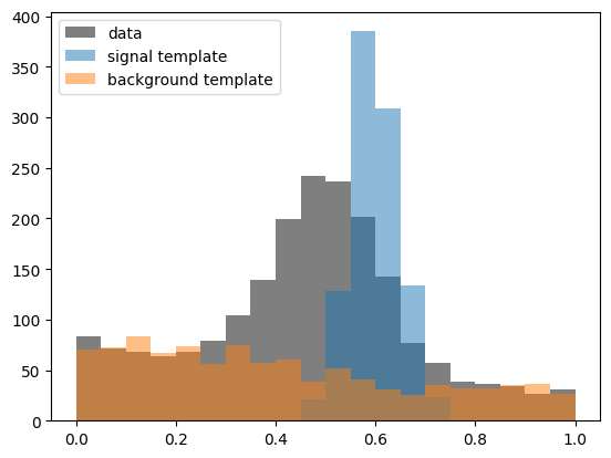
We explore this on a toy example. We want to fit a peak over smooth background using templates. The sample which provides a template for the peak is distorted. Its mean is shifted and it also too narrow. We want to fit the yield of this peak under these conditions.
In practice, this situation is common. The simulation is a good, but not perfect approximation of reality. Template fits could work very well in these situations if we find a way to fit a slightly distorted template instead of the raw one. For this to work, the distortion has to be a simple function, for example, an affine transformation like in this case. Then, the transformation can be fitted together with the yields. The parameters of the transformation are nuisance parameters. Note that the uncertainty of the fitted yield will always increase when such a transformation has to be estimated from the data as well.
The catch
The idea to fit a transformed template is straight-forward, but there is a catch. Standard minimizers employed in HEP use a method based on gradient descent, and the gradient is computed numerically using a finite-difference formula. These minimizers only work correctly if the function to minimize is smooth: its first and second derivatives must be smoothly varying. But this is not the case the in the outlined approach, because the transformation will cause points from the samples that form the template to migrate from bin to bin. This causes jumps in the objective function and thus discontinuities in the derivatives. MINUIT does not like that at all. It can fail to converge, get stuck in a local minimum, or may report convergence to a point which is not a minimum. All of these outcomes are bad. The following cells demonstrate how MINUIT fails on such a fit. As objective function, we use the transformed approximate likelihood for template fits that we derived in our paper (implemented in template_chi2_da).
def model(s, b, offset, scale): mu_st_sample = np.mean(st_sample) st_sample_modified = scale * (st_sample - mu_st_sample) + mu_st_sample + offset template_s_modified = np.histogram(st_sample_modified, bins=xe)[0]# a small constant is added to avoid dividing by zero ts = template_s_modified / (np.sum(template_s_modified) +1e-6) tb = template_b / np.sum(template_b) mu = s * ts + b * tb mu_var = s * ts**2+ b * tb**2return mu, mu_vardef objective(s, b, offset, scale): mu, mu_var = model(s, b, offset, scale)return template_chi2_da(n_data, mu, mu_var)# if errordef and ndata on the objective are set,# iminuit computes the chi2 gof test statistic for usobjective.errordef = Minuit.LEAST_SQUARESobjective.ndata =len(xe) -1m = Minuit(objective, s=1000, b=1000, offset=0, scale=1)m.limits["s", "b"] = (0, None)m.limits["scale"] = (0.01, 2.5)m.limits["offset"] = (-0.2, 0.2)m.migrad()
Migrad
FCN = 499 (χ²/ndof = 31.2)
Nfcn = 296
EDM = 2.72e-12 (Goal: 0.0002)
Valid Minimum
Below EDM threshold (goal x 10)
No parameters at limit
Below call limit
Hesse ok
Covariance accurate
Name
Value
Hesse Error
Minos Error-
Minos Error+
Limit-
Limit+
Fixed
0
s
494
33
0
1
b
1.51e3
0.05e3
0
2
offset
-9.0380e-3
0.0033e-3
-0.2
0.2
3
scale
999.17e-3
0.31e-3
0.01
2.5
s
b
offset
scale
s
1.08e+03
-0.4e3 (-0.299)
-2.648168e-6 (-0.025)
-124.42e-6 (-0.012)
b
-0.4e3 (-0.299)
2.02e+03
3.171095e-6 (0.022)
149.02e-6 (0.011)
offset
-2.648168e-6 (-0.025)
3.171095e-6 (0.022)
1.06e-11
0.497e-9 (0.498)
scale
-124.42e-6 (-0.012)
149.02e-6 (0.011)
0.497e-9 (0.498)
9.39e-08
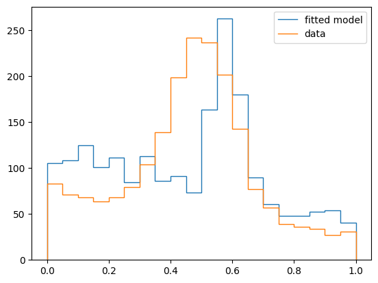
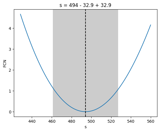
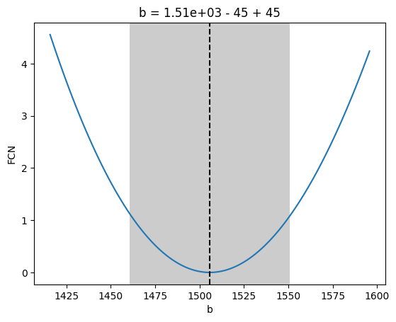
MINUIT reports successful convergence, but signal and background yields are far from the truth. Also, the chi2/ndof ratio is far from 1. We can see that this a poor fit by drawing the fitted model and by looking at the profile-likelihood for each parameter.
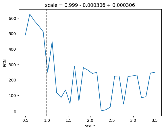
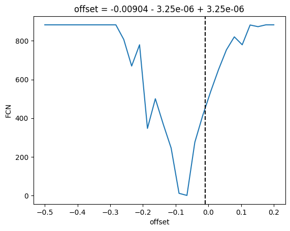
plt.figure()m.draw_profile("s")plt.figure()m.draw_profile("b")# ignore some iminuit warnings about failing to converge during profile computationwith warnings.catch_warnings(): warnings.simplefilter("ignore", IMinuitWarning) plt.figure() m.draw_mnprofile("scale", bound=(0.5, 3.5)) plt.figure() m.draw_mnprofile("offset", bound=(-0.5, 0.2))
We can see in the profile that we are not in the global minimum, which is near offset = -0.1 and scale = 2.2.
Solution
Two solutions come to mind, both have caveats. I explore one below, which I consider to be the simpler one. The second solution is to replace the transformed template by a kernel density estimate. This would lead to additional hyperparameters introduced by the kernel density estimation, which would need to be carefully chosen for each problem, and require the derivation of a new complicated likelihood function for this case.
Use a global derivative-free minimizer and bootstrapping
Since we cannot use a local minimizer which uses gradients for our objective function, we switch to a global derivative-free minimizer. Global derivative-free minimizers require many more function calls than standard local minimizers like MINUIT’s MIGRAD, and this number moreover scales quadratically with the number of fitted parameters. Fortunately, our objective function is relative fast to compute and does not have many parameters, so global minimization is feasible. In the following, I apply the differential_evolution algorithm from scipy to this problem.
Optimization terminated successfully.
chi2/ndof = 1.0
s         = 1017
b         = 987
offset    = -0.09
scale     = 2.0
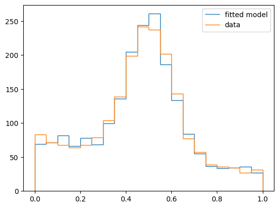
This looks great! We got an excellent chi2/ndof ratio and the fitted model agrees well with the data. Our idea works, and the global minimizer did not take too much time either.
Now we need to address the next challenge: we also want to know the parameter uncertainties. We cannot use the usual technique of inverting the appropriately scaled Hesse matrix of the objective function at the minimum to get the covariance matrix, because this would again require a numerical computation of second derivatives.
I will nevertheless attempt to compute the covariance matrix with Minuit’s HESSE algorithm to see what happens.
m.values = r.xm.hesse()
External
FCN = 15.5 (χ²/ndof = 1.0)
Nfcn = 9332
EDM = 0.0125 (Goal: 0.0002)
INVALID Minimum
ABOVE EDM threshold (goal x 10)
No parameters at limit
Below call limit
Hesse ok
Covariance accurate
Name
Value
Hesse Error
Minos Error-
Minos Error+
Limit-
Limit+
Fixed
0
s
1.02e3
0.04e3
0
1
b
990
40
0
2
offset
-87.39e-3
0.14e-3
-0.2
0.2
3
scale
1.9848
0.0015
0.01
2.5
s
b
offset
scale
s
1.85e+03
-0.7e3 (-0.380)
4.261e-6
-185.2e-6 (-0.003)
b
-0.7e3 (-0.380)
1.7e+03
-28.018e-6 (-0.005)
-217.3e-6 (-0.003)
offset
4.261e-6
-28.018e-6 (-0.005)
2.08e-08
0.050e-6 (0.230)
scale
-185.2e-6 (-0.003)
-217.3e-6 (-0.003)
0.050e-6 (0.230)
2.29e-06
The minimum is reported as invalid, that is suspicious. HESSE reports success, but the uncertainties on offset and scale are suspiciously small. We should not trust this result. This is one of the possible outcomes if the second derivatives are not well-defined bad. In other cases, HESSE may fail or report that the covariance matrix had to be forced to be positive definite.
Since this does not work, we employ the bootstrap technique, using the resample library. This library provides a function which readily computes the covariance for a function that depends on a single dataset, but we have a more complicated case here. We need to resample three samples simultaneously, which have different sizes, the data sample and the two samples that generate the templates. We use the “extended” resampling method to also vary the sizes of these samples, which is usually the correct thing in high-energy physics, but not how the standard bootstrap in the literature works.
# function which does the whole estimation; taking samples as input and# returning parameters of interest as outputdef fit(x_sample, st_sample, bt_sample): n_data = np.histogram(x_sample, bins=xe)[0] template_b = np.histogram(bt_sample, bins=xe)[0]def model(s, b, offset, scale): mu_st_sample = np.mean(st_sample) st_sample_modified = scale * (st_sample - mu_st_sample) + mu_st_sample + offset template_s_modified = np.histogram(st_sample_modified, bins=xe)[0]# a small constant is added to avoid dividing by zero ts = template_s_modified / (np.sum(template_s_modified) +1e-6) tb = template_b / np.sum(template_b) mu = s * ts + b * tb mu_var = s * ts**2+ b * tb**2return mu, mu_vardef objective(s, b, offset, scale): mu, mu_var = model(s, b, offset, scale)return template_chi2_da(n_data, mu, mu_var) r = differential_evolution(lambda x: objective(*x), bounds=((0, 2000), (0, 2000), (-0.2, 0.2), (0.5, 3.5)), polish=False, seed=1, )assert r.successreturn r.xnumber_of_bootstrap_samples =20kwargs = {"size": number_of_bootstrap_samples, "method": "extended", "random_state": 1}results = []for xs, sts, bts inzip( resample(x_sample, **kwargs), resample(st_sample, **kwargs), resample(bt_sample, **kwargs),): xb = fit(xs, sts, bts) results.append(xb)cov = np.cov(results, rowvar=False)for name, val, err inzip(m.parameters, r.x, np.diag(cov) **0.5):print(f"{name} = {val:.2f} +/- {err:.2f}")
s = 1016.88 +/- 71.60
b = 987.33 +/- 51.06
offset = -0.09 +/- 0.00
scale = 1.98 +/- 0.16
The calculation takes a while but eventually completes. We now find larger uncertainties compared to the HESSE estimate above, which essentially treated the transform like it was fixed. We can see that the increase in the uncertainties indeed originates from the fitted transform, if we repeat the bootstrap with fixed the transformation parameters.
At least in some cases, it is possible to fit distorted templates and estimate the distortion parameters as nuisance parameters, and get good results with modest effort. The solution described here will work best if the components in the mixture are well separated and if the same distortion can be applied to all templates (for example, because it models a calibration mismatch).
In the following cases, this method will introduce large uncertainties on the fitted yields:
the components are strongly overlapping
different distortions are needed for each template
the distortion function is very flexible and has many parameters
In some of these difficult cases, reasonable results may be attainable if the distortion parameters are further constrained with penalty terms, that prevent the distortion function from diverging too much from the identity.